
Trading on a Rigged Game: Outcome Manipulation in Prediction Markets
Proceedings of the Twenty-Fifth International Joint Conference on Artificial Intelligence. Pages 158-163.
Abstract
Prediction markets are popular mechanisms for aggregating information about a future event. In situations where market participants may significantly influence the outcome, running the prediction market could change the incentives of participants in the process that creates the outcome. We propose a new game-theoretic model that captures two aspects of real-world prediction markets: (1) agents directly affect the outcome the market is predicting, (2) some outcome-deciders may not participate in the market. We show that this game has two types of equilibria: When some outcome-deciders are unlikely to participate in the market, equilibrium prices reveal expected market outcomes conditional on participants' private information, whereas when all outcome-deciders are likely to participate, equilibria are collusive — agents effectively coordinate in an uninformative and untruthful way.
- [Abernethy and Frongillo, 2012] J. Abernethy and R. Frongillo. A characterization of scoring rules for linear properties. COLT, 2012.
- [Berg and Rietz, 2006] J. Berg and T. Rietz. The Iowa elec- tronic markets: Stylized facts and open issues. Information Markets: A New Way of Making Decisions, pages 142- 169, 2006.
- [Berg et al., 2008] J. Berg, R. Forsythe, F. Nelson, and T. Ri- etz. Results from a dozen years of election futures markets research. Handbook Exp. Econ. Res., 1:742-751, 2008.
- [Boutilier, 2012] C. Boutilier. Eliciting forecasts from self- interested experts: scoring rules for decision makers. Proc. AAMAS, 2:737-744, 2012.
- [Brahma et al., 2012] A. Brahma, M. Chakraborty, S. Das, A. Lavoie, and M. Magdon-Ismail. A Bayesian market maker. In Proc. ACM EC, pages 215-232, 2012.
- [Chakraborty et al., 2013] M. Chakraborty, S. Das, A. Lavoie, M. Magdon-Ismail, and Y. Naamad. In- structor rating markets. In Proc. AAAI, pages 159-165, 2013.
- [Chen and Pennock, 2007] Y. Chen and D. Pennock. A util- ity framework for bounded-loss market makers. In Proc. UAI, pages 49-56, 2007.
- [Chen et al., 2009] Y. Chen, S. Dimitrov, R. Sami, D. Reeves, D. Pennock, R. Hanson, L. Fortnow, and R. Gonen. Gaming prediction markets: Equilibrium strategies with a market maker. Algorithmica, pages 1-40, 2009.
- [Chen et al., 2011a] Y. Chen, X. Gao, R. Goldstein, and I. Kash. Market manipulation with outside incentives. In Proc. AAAI, 2011.
- [Chen et al., 2011b] Y. Chen, I. Kash, M. Ruberry, and V. Shnayder. Decision markets with good incentives. In Proc. WINE, pages 89-100, 2011.
- [Cowgill and Zitzewitz, 2015] B. Cowgill and E. Zitzewitz. Corporate prediction markets: Evidence from Google, Ford, and Firm X. Review Econ. Studies, 82(4):1309- 1341, 2015.
- [Das, 2008] S. Das. The effects of market-making on price dynamics. In Proc. AAMAS, May 2008.
- [Dimitrov and Sami, 2010] S. Dimitrov and R. Sami. Com- position of markets with conflicting incentives. In Proc. ACM EC, pages 53-62, 2010.
- [Foster and Viswanathan, 1996] F. Foster and S. Viswanathan. Strategic trading when agents fore- cast the forecasts of others. J. Fin., 51:1437-1478, 1996.
- [Fudenberg and Tirole, 1991] D. Fudenberg and J. Tirole. Perfect Bayesian equilibrium and sequential equilibrium. J. Econ. Theory, 53(2):236-260, 1991.
- [Gao et al., 2013] X. Gao, J. Zhang, and Y. Chen. What you jointly know determines how you act: Strategic interac- tions in prediction markets. In Proceedings of the four- teenth ACM conference on Electronic commerce, pages 489-506. ACM, 2013.
- [Glosten and Milgrom, 1985] L. Glosten and P. Milgrom. Bid, ask and transaction prices in a specialist market with heterogeneously informed traders. J. Fin. Econ., 14:71- 100, 1985.
- [Gneiting and Raftery, 2007] T. Gneiting and A. Raftery. Strictly proper scoring rules, prediction, and estima- tion. Journal of the American Statistical Association, 102(477):359-378, 2007.
- [Hanson and Oprea, 2009] R. Hanson and R. Oprea. A ma- nipulator can aid prediction market accuracy. Economica, 76(302):304-314, 2009.
- [Hanson et al., 2006] R. Hanson, R. Oprea, and D. Porter. Information aggregation and manipulation in an experi- mental market. J. Econ. Beh. and Org., 60:449-459, 2006.
- [Hanson, 1999] R. Hanson. Decision markets. IEEE Intelli- gent Systems, 14(3):16-19, 1999.
- [Hanson, 2003] R. Hanson. Combinatorial information mar- ket design. Information Systems Frontiers, 5(1):107-119, 2003.
- [Hanson, 2007a] R. Hanson. Logarithmic market scoring rules for modular combinatorial information aggregation. J. Prediction Markets, 1(1):3-15, 2007.
- [Hanson, 2007b] R. Hanson. The Policy Analysis Market (a thwarted experiment in the use of prediction markets for public policy). Innovations, 2(3):73-88, 2007.
- [Holden and Subrahmanyam, 1992] C. Holden and A. Sub- rahmanyam. Long-lived private information and imperfect competition. J. Fin., 47:247-270, 1992.
- [Huang and Shoham, 2014] E. Huang and Y. Shoham. Price manipulation in prediction markets: analysis and mitiga- tion. In Proc. AAMAS, pages 213-220, 2014.
- [Kyle, 1985] A. Kyle. Continuous auctions and insider trad- ing. Econometrica, 53(6):1315-1336, 1985.
- [Miller et al., 2005] N. Miller, P. Resnick, and R. Zeck- hauser. Eliciting Informative Feedback: The Peer- Prediction Method. Management Science, 5(9):1359- 1373, Sept. 2005.
- [Ostrovsky, 2012] M. Ostrovsky. Information aggregation in dynamic markets with strategic traders. Econometrica, 80(6):2595-2647, 2012.
- [Othman and Sandholm, 2010] A. Othman and T Sandholm. Decision rules and decision markets. In Proc. AAMAS, pages 625-632, 2010.
- [Peterson and Krug, 2015] J. Peterson and J. Krug. Augur: a decentralized, open-source platform for prediction mar- kets. arXiv preprint arXiv:1501.01042, 2015.
- [Rhode and Strumpf, 2006] P. Rhode and K. Strumpf. Ma- nipulating political stock markets: A field experiment and a century of observational data. University of Arizona, mimeo, 2006.
- [Rothschild and Sethi, 2015] D. Rothschild and R. Sethi. Trading strategies and market microstructure: Evidence from a prediction market. Available at SSRN 2322420, 2015.
- [Shi et al., 2009] P. Shi, V. Conitzer, and M. Guo. Prediction mechanisms that do not incentivize undesirable actions. In Proc. WINE, 2009. [Stiglitz, July 31 2003]
- J. Stiglitz. Terrorism: There's no fu- tures in it. Los Angeles Times, July 31, 2003.
- [Wolfers and Zitzewitz, 2004] J. Wolfers and E. Zitzewitz. Prediction markets. J. Econ. Perspectives, 18(2):107-126, 2004.
References were extracted automatically from the PDF and may contain errors.
Full text extracted automatically from the PDF; figures, tables and equations may differ. The PDF is the version of record.
1 Introduction
Prediction markets are widely used tools for aggregating and disseminating private information on some future event, dispersed among a potentially diverse crowd. However, attention is seldom paid in the literature to the possibility that market participants might have some degree of control on the outcome of the forecast event, and hence the presence of a prediction market may make agents affecting the outcome act differently than they otherwise would. In fact, sometimes it is this very power to affect outcomes that gives agents the informational edge that such markets get their value from.
Consider three real-world examples where prediction (or betting) markets have demonstrated their forecasting ability: politics [Berg et al., 2008], sporting events [Wolfers and Zitzewitz, 2004], and software product releases [Cowgill and Zitzewitz, 2015]. In each of these cases, it is easy to see how a prediction market may distort outcomes: A congressional staffer or member of congress may know more about the probable result of a key vote than the general public, but she is also in a position to influence this result. A referee or player has substantial ability to influence the outcome of a sporting event. A software engineer has the potential to delay (or speed up) the release of a product. When such outcome manipulation incentives are present, it is natural to ask two questions: (1) Are the actions of the outcome-deciders still truthful, i.e. do they take the same actions that they would in the absence of the prediction market? (2) Are market prices still informative, i.e. how much do they still tell us about the realized outcome?
While it is acknowledged that prediction markets have value as aids in making business and policy decisions, they have gone through cycles of hype and bust for reasons that include regulatory concerns about manipulation. The emblematic anecdote about this problem is the failure of DARPA's proposed Policy Analysis Markets which were caricatured in the media as "terrorism futures" [Hanson, 2007b; Stiglitz, July 31 2003]. There are obviously markets that will not work but stock and futures markets have been used for a long time as forecasting tools, and prediction markets are similar in essence. The key is to understand when markets may be prone to manipulation and how much to trust them.
1.1 Contributions
A model for outcome manipulation: We propose a new model for studying manipulative behavior that captures two aspects of real-world prediction markets: (1) agents directly affect the forecast event, (2) some of the agents who have influence over the outcome may not participate in the prediction market (e.g. employees who have an impact on the outcome of a product launch typically would not all take part in the company's in-house prediction market for its release date). In markets where an individual has a small effect on the outcome, agents' incentives for manipulation are likely to be weak. With this in mind, we mainly focus on a two-stage game-theoretic model of a market with two players, Alice and Bob, who affect the outcome and can also trade on it (Sections 2 and 3), and then discuss how our insights extend to models with more outcome-deciders in Section 4.
In the first stage of the game, Alice and Bob each receive a private signal about the underlying entity, and then they have the opportunity to participate sequentially, once each, in a prediction market mediated by a market scoring rule or MSR [Hanson, 2007a]. However, depending on his type, there is a probability that Bob may not participate in trading. In the second stage, the two players simultaneously take actions which we term "votes" for convenience, although in general they model each participant's role in determining the outcome. 1 The payoffs from the first-stage prediction market are determined by a simple function of the stage two votes. If Bob has not traded, his vote is consistent with his private signal, otherwise he is strategic; the first mover Alice is always strategic.
Our model directly captures the experiments of Chakraborty et al. [2013] where prediction markets with student participants were used to forecast the fraction of "up" (vs "down") ratings given by students to course instructors. Moreover, Augur, a recently launched "decentralized, open-source platform for prediction markets" [Peterson and Krug, 2015], is a real-world mechanism with manipulation incentives similar to those in our model: A consensus, computed from votes cast by participants called "reporters", serves as a proxy for the payoff-deciding ground truth of a market on which these reporters can also wager.
A dichotomy of equilibria: Our main result is that the equilibria of our game-theoretic model can be cleanly categorized into two types, depending on Bob's probability of participation in the trading stage. Below a threshold on this probability, say ˜ p (a function of the MSR used and the signal structure), we call the equilibrium a low participation probability equilibrium (LPPE), and above ˜ p, we call it a high participation probability equilibrium (HPPE). In a LPPE, Alice essentially predicts Bob's vote, and then bases her trading on the optimal combination of her own and Bob's votes, and the prediction market price is reflective of the expected outcome. In a HPPE, on the contrary, Alice effectively expects Bob to enter and collude with her, and she chooses a prediction market price that allows Bob and her to "split the profit". We summarize the qualitative implications of our result in Section 3.1.
1.2 Related work
The market microstructure we use here is a market scoring rule (MSR), introduced by Hanson [2003] and expanded upon by many researchers ([Chen and Pennock, 2007; Chen et al., 2009; Gao et al., 2013] etc.). Incentives for manipulation in prediction markets may arise in a number of ways. There is a plethora of literature on price manipulation - tampering with the market price owing to some extra-market incentives ([Hanson et al., 2006; Rhode and Strumpf, 2006; Hanson and Oprea, 2009; Boutilier, 2012; Dimitrov and Sami, 2010; Chen et al., 2011a; Huang and Shoham, 2014]), e.g. a politically motivated manipulator might make a large investment in an election prediction market to make one of the candidates appear stronger [Rothschild and Sethi, 2015]; a related body of work pertains to decision markets - a collection of contingent markets set up to predict the outcomes of different decisions such that only markets contingent on decisions that are taken pay off, the rest being voided [Hanson, 1999; Othman and Sandholm, 2010; Chen et al., 2011b]. The type of manipulation that we are concerned with is outcome manipulation where an agent can take an action that partially influences the outcome to be predicted (e.g. [Berg and Rietz, 2006; Shi et al., 2009]), and we study it in a new model.
1 For example, for a product release date prediction market, a (binary) private signal could stand for whether an agent knows / believes she is capable of contributing her share in making sure that the launch is on time; her (binary) vote in this case would indicate whether she actually plays her part honestly.
The second major body of related literature comes from theoretical finance and market microstructure. Kyle [1985], followed by Holden and Subrahmanyam [1992], Foster and Viswanathan [1996] etc., studied the effect of informed "insider(s)" on market price; Glosten and Milgrom [1985] presented another view of how asymmetric information affects price formation, and their model has been adapted for market making in prediction markets [Das, 2008; Brahma et al., 2012]. Ostrovsky [2012] recently examined information aggregation with differentially informed traders under both Kyle's pricing model and market scoring rules. Again, in all of these models, the market outcome is assumed to be exogenously determined, unlike in ours.
2 Model and definitions
Let ⌧ 2 T denote the unobservable "true value" of the random variable on which the voting system and its associated prediction market are predicated. At t = 0, the two agents, Alice and Bob (A and B in subscripts), receive private signals sA↪ sB 2 ⌦ = ¶0↪ 1♦ respectively. The signal structure, comprising the prior distribution Pr(⌧) on the true value and the conditional joint distribution Pr(sA↪ sB♣⌧) of the private signals given the true value, is common knowledge.
Let q0(·) denote Alice's posterior probability that Bob received the signal sB = 0, given her own signal and common knowledge, i.e. q0(s) , Pr (sB = 0♣sA = s) 8s 2 ¶0↪ 1♦. We ignore the uninteresting special cases q0 2 ¶0↪ 1♦ corresponding to Alice having no uncertainty about her peer's private signal. Although we need no further assumptions on the signal structure for our main result (Theorem 1), it is worthwhile to define here the property of stochastic relevance [Miller et al., 2005] which is a necessary assumption for one of our important corollaries.
Definition 1. For binary random variables si↪ sj 2 ¶0↪ 1♦, sj is said to be stochastically relevant for si if and only if the posterior distribution of si given sj is different for different realizations of sj, i.e. if and only if Pr(si = 0♣sj = 0) 6= Pr(si = 0♣sj = 1).
We now describe the rules of the two-stage game comprising the market and voting mechanisms. We will call this the trading-voting game.
Stage 1 (market stage): The market price at any time-step t is public, the starting price at t = 0 being p0 which is the market designer's baseline estimate of the outcome (equal to the final gross payoff per unit of the security).
The prediction market is implemented using a market scoring rule (MSR) [Hanson, 2007a] with the underlying strictly proper scoring rule s(r↪ !), where ! is the outcome to be forecast - in our model, determined by Stage 2 (see below) - and r is an agent's forecast / report on it; strict propriety, by definition, implies that if a forecaster is promised an ex post compensation of s(r↪ !), then the only way she can maximize her subjective expected compensation is by reporting her expectation of the random variable !. For a clean analysis, we shall focus on strictly proper rules for eliciting the expectation of the random variable ! 2 [0↪ 1], satisfying some regularity and smoothness conditions [Gneiting and Raftery, 2007; Abernethy and Frongillo, 2012]:
where f(·) is a continuous, finite, strictly convex function on [0↪ 1]; its first derivative f 0 (·) is continuous, monotonically increasing, and finite on [0↪ 1] except possibly that f 0 (0) = -1 or f 0 (1) = 1, with limr!0 f 0 (r)r = limr!1 f 0 (r)(1 - r) = 0; the second derivative f 00 (·) is positive on [0↪ 1] and finite in (0↪ 1). Additionally, we need the function to have the following symmetry:
Henceforth, we shall refer to (market) scoring rules possessing all the above properties as symmetric well-behaved (market) scoring rules. This covers a large family of MSRs including three of the most widely used and studied - logarithmic (LMSR), quadratic (QMSR), and spherical (SMSR) - defined in terms of their respective convex functions as:
At t = 1, Alice interacts with the market maker and changes the price to pA. At t = 2, Bob has an opportunity to trade but may not show up with a (common-knowledge) probability ⇡ 2 [0↪ 1] called Bob's non-participation probability; if he does trade, he changes the price to pB. Regardless of whether Bob trades, the market terminates after t = 2. Stage 2 (voting stage): In this stage, Alice and Bob simultaneously declare their "votes" vA↪ vB 2 ⌦ = ¶0↪ 1♦ respectively. Taking part in Stage 2 is mandatory for both agents. We define truthful voting as declaring one's private signal as one's vote, i.e. vk = sk, k 2 ¶A↪B♦. We assume that, if Bob did not trade in Stage 1, he votes truthfully, and we call such a Bob HONEST. Any agent participating in the prediction market is Bayesian, strategic, and risk-neutral. Hence, if
Bob trades, we refer to him as STRATEGIC Bob.
The market outcome is given by the average vote v = (vA + vB) ◁2 2 ¶0↪ 12 ↪ 1♦. Alice and Bob's ex post net payoffs of are respectively
Bob does not strategically decide whether to take part in the market, it is determined extraneously - the proclivity to trade can be viewed as one of the components of Bob's type, the other being his private signal sB. Here, HONEST Bob models agents whose outcome-deciding actions remain unaltered by the introduction of the prediction market.
3 Equilibrium analysis
The solution concept we use for the trading-voting game described in Section 2 is the perfect Bayesian equilibrium (PBE), a refinement of Nash equilibria for Bayesian games [Fudenberg and Tirole, 1991]. In this section, we present the main theorem, its supporting lemmas and main corollaries, and defer full proofs to a longer version of the paper.
Our first result formalizes the intuition that, if Alice pulls the market price down (resp. up) from its initial value, she is "forecasting" that the final outcome will be lower (resp. higher) than the market's initial estimate and hence it is in her best interest to do everything in her power to ensure a low (resp. high) average vote - this is because her payoff is higher for a prediction closer to the realized outcome.
Lemma 1. For the trading-voting game described in Section 2, if the prediction market has a starting price p0 2 (0↪ 1) at t = 0, and (pA↪ vA) denotes Alice's combined action in the two-stage game, i.e. her report-vote pair, then
- ÷ for any pA < p0, (pA↪ 0) strictly dominates (pA↪ 1);
- ÷ for any pA > p0, (pA↪ 1) strictly dominates (pA↪ 0); and
- ÷ she is indifferent between the actions (p0↪ 0) and (p0↪ 1).
This result holds regardless of Bob's report-vote pair (pB↪ vB).
Lemma 1 implies that immediately after Alice has traded, anyone can infer that vA = 0 deterministically if pA < p0, vA = 1 deterministically if pA > p0, and that she is equally likely to vote 0 or 1 if pA = p0, which is equivalent to not trading with the market maker. As soon as STRATEGIC Bob arrives to trade, he acquires all the information relevant to his decision making procedure that the rules of the game allow him to have (pA and vA). Thus, STRATEGIC Bob makes his trading and voting decisions (pB↪ vB) simultaneously.
The next step is to determine Bob's best response to Alice's Stage 1 action. For this, we need to define quantities that we call the lower and upper thresholds pL and pH :
For any symmetric, well-behaved scoring rule, we can show that pH = 1 - pL. For LMSR, QMSR, and SMSR, pL is 0▷2, 0▷25, and 0▷2725 respectively.
Lemma 2. For the trading-voting game described in Section 2, where the market is implemented with a symmetric well-behaved market scoring rule with lower and upper thresholds pL↪ pH , and has a starting price p0 2 (0↪ 1),
- ÷ if pA < p0, then STRATEGIC Bob's best-response vote is vB = 1 (resp. vB = 0) if pA < pL (resp. pA > pL) but he is indifferent between the two possible voting choices if pA = pL; his accompanying price-report is pB = vB 2 ;
- ÷ if pA > p0, then STRATEGIC Bob's best-response vote is vB = 1 (resp. vB = 0) if pA < pH (resp. pA > pH ) but he is indifferent between the two possible voting choices if pA = pH ; his accompanying pB is 1+vB 2 ;
- ÷ if pA = p0, then STRATEGIC Bob's best-response vote is vB = 0 (resp. vB = 1) if p0 > 1◁2 (resp. p0 < 1◁2) but he is indifferent if p0 = 1◁2, and his accompanying price-report is pB = 1◁2+vB 2 .
This result is independent of Bob's private signal sB.
pL, pH , and p0 are points of transition in agent behavior: Bob's best response is to "disagree with" Alice's voting choice (revealed through pA) in Stage 2 if Alice's price-report lies in either of the "outer" sub-intervals [0↪min(p0↪ pL)) or (max(p0↪ pH )↪ 1], and to "agree with" her otherwise; for pA 6= p0, STRATEGIC Bob knows what the market outcome v is going to be, so he can make a perfect forecast pB = v.
This fully characterizes how the game unfolds after Alice has taken her Stage 1 action. Now, the final step towards completing the equilibrium specification is to figure out Alice's best-response price-report pA, based on q0, ⇡, and her knowledge of Lemmas 1 and 2. In the extreme case ⇡ = 0, when Bob's (strategic) participation is certain, it is natural to conjecture that Alice as the first mover will invite Bob to create a "fake world" with little connection to their private signals; at the other end of the spectrum (⇡ = 1) where Alice is sure that Bob is HONEST, we expect her action to shed some light on her posterior belief about Bob's signal. Theorem 1 tells us that there exists some critical value of Bob's non-participation probability at which a switch between partially revealing and collusive equilibria occur. 2
Theorem 1. For any value of Bob's non-participation probability ⇡ 2 (0↪ 1) and Alice's posterior belief q0 2 (0↪ 1), the trading-voting game described in Section 2 has a perfect Bayesian equilibrium with the following attributes: For every q0, there exists a fixed value of Bob's non-participation probability, say ⇡c(q0), which we call the "crossover" probability (dependent on the MSR), on either side of which the equilibria are qualitatively different. We call the sub-interval ⇡ < ⇡c the high participation probability (HPP) equilibrium domain, and the sub-interval ⇡ > ⇡c the low participation probability (LPP) equilibrium domain.
÷ In a HPP equilibrium:
- In Stage 1, Alice moves the market price to pA = pL if q0 > 12 , and to pA = pH if q0 < 12 ; STRATEGIC Bob's priceupdate is pB = 0 if pA = pL, and pB = 1 if pA = pH .
- In Stage 2, Alice votes vA = 0 if she set pA = pL, vA = 1 if pA = pH ; STRATEGIC Bob votes vB = 0 if he set pB = 0, and vB = 1 if he set pB = 1.
÷ In a LPP equilibrium:
- In Stage 1, Alice's price-report pLPP A is equal to her posterior expectation of the market liquidation value (average vote) given the parameters ⇡↪ q0 and her report pLPP A , i.e. pLP P A = E ⇥v♣⇡↪ q0↪ pA = pLPP A ⇤. Moreover, pLPP A < 12 if q0 > 12 , pLPP A > 12 if q0 < 12 . STRATEGIC Bob's priceupdate is pB = 0 if pL pA 12 , pB = 1 if 12 < pA pH , and pB = 12 otherwise.
- In Stage 2, Alice votes vA = 0 if pA > 12 , vA = 1 if pA < 12 ; STRATEGIC Bob votes vB = 0 if pA 2 ⇥pL↪ 12 ⇤ [ (pH ↪ 1⇤, vB = 1 otherwise.
More specifically, pLPP A is one of θ0↪0 = ⇡(1-q0) 2 , θ0↪1 = 1-⇡q0 2 , θ1↪0 = 1+⇡(1-q0) 2 , θ1↪1 = 1- ⇡q0 2 , where 0 < θ0↪0 < θ0↪1 < 12 < θ1↪0 < θ1↪1 < 1. Table 1 presents the crossover probability ⇡c as a function of q0 for sub-classes of symmetric well-behaved MSRs defined on the basis of the value of pL, and also the values of Alice's equilibrium price-reports in the LPP domain, for q0 1◁2. For q0 > 1◁2, the results are symmetric, hence omitted. In the HPP domain, pPBE A is pH whenever q0 < 1◁2, and pL whenever q0 > 1◁2. At ⇡ = ⇡c, then Alice is indifferent between her LPP and HPP pricereports although the values of these reports are, in general, distinct. Below, we outline the proof of Theorem 1.
2 We present our results for p0 = 12 , which corresponds to starting the market at a uniform "prior" - a standard practice in prediction markets.
| q0 | ⇡c(q0) of pL | pP BE A for LPP Range of pL < 14 | ||
|---|---|---|---|---|
| Range < 14 | ≥ 14 ⇡⇤ 1 (q0) | θ1↪0 | ≥ 14 θ1↪0 | |
| 0 < q0 < 2pL q0 = 2pL 2pL < q0 < 12 q0 = 12 | ⇡⇤ 1 (q0) 1 2pL q0 4pL | ⇡⇤ 1 (q0) ⇡⇤ 1 (q0) ⇡⇤ | NA θ1↪1 θ1↪1 / θ0↪0 | θ1↪0 θ1↪0 θ1↪0 |
Proof sketch Owing to linearity, Alice's expected payoff with respect to her uncertainty in Bob's participation and signal is equal to her payoff function evaluated at her expected outcome. Hence, using Lemmas 1 and 2, we can show that this expected payoff function is a piecewise continuous function of pA consisting of segments of the "component" functions RA(pA↪ 12 ↪ 0↪ 1), RA(pA↪ 12 ↪ 0↪ 0), RA(pA↪ 12 ↪ 1↪ 1), and RA(pA↪ 12 ↪ 1↪ 0) over the sub-intervals (0↪ pL), (pL↪ 12 ], ( 12 ↪ pH ), (pH ↪ 1) respectively, with jump discontinuities at pL↪ pH . The global maxima of these components in [0↪ 1] are located respectively at θ0↪1, θ0↪0, θ1↪1, and θ1↪0, which depend on ⇡ and q0. However, for any given q0 (and pL↪ pH ), depending on the value of ⇡, the global maximum of one of these components might lie outside the sub-interval in which that component is applicable so that the local suprema of some of the segments may lie at a threshold pL or pH . Taking these issues into account, we can determine the local suprema of the four segments and compare them to find the pA that maximizes Alice's expected payoff; the rest of the theorem follows from Lemmas 1 and 2, with the restriction that vB = 0 if pA = pL and vB = 1 if pA = pH . ⇤
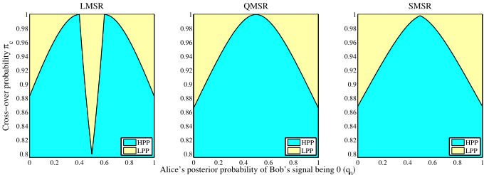
Figure 1 depicts the crossover probability ⇡c as a function of q0 for each of the three selected MSRs. An interesting point is that for LMSR, when 0▷4 < q0 < 0▷6, which is a region of "high" uncertainty in Alice's posterior about Bob's private signal, ⇡c actually decreases with Alice's increasing uncertainty, i.e. the partially revealing LPP domain is realized for lower values of Bob's non-participation probability than for the other MSRs. This is a peculiarity of any MSR with pL < 1◁4 as opposed those with pL ≥ 1◁4.
3.1 Implications
Private signal revelation: STRATEGIC Bob's report-vote pair is fully determined by Alice's report and does not depend on sB; there is no guarantee that Alice's vote will be truthful either, even in a LPP equilibrium (in general, she is likely to guess which way Bob will vote and vote the same way). However, if we invoke the assumption of stochastic relevance (Definition 1), then we can use pA to uncover sA.
Corollary 1. If Alice's signal sA is stochastically relevant for Bob's signal sB, then the value of sA can be recovered from Alice's price-report in a LPP equlibrium pLPP A = θu↪v(⇡↪ q0), u↪ v 2 ¶0↪ 1♦, regardless of whether vA = sA.
In other words, the very possibility of Bob not trading but voting truthfully engenders a situation (LPP domain) in which Alice, though strategic, is forced to indirectly divulge her private information! This has major implications for the value of prediction markets in situations where the "voting" or outcome-deciding actions of individuals are already assumed to be truthful and the designer would prefer not to introduce incentives that make them untruthful just because they added a trading platform. Corollary 1 suggests that, for an MSR-based prediction market, manipulators run the risk of having their cover blown when some fraction of the outcomedeciders refrain from market participation and are truthful in their outcome-affecting actions.
In a HPP equilibrium, pA can only tell us whether q0 > 12 (if pA = pL) or q0 < 12 (if pA = pH ), and is insufficient for recovering sA without further assumptions.
HPP profit sharing: The HPP equilibria are a world where collusion appears with Alice as the "leader" picking the vote that both will coordinate on, and moving the price to just the level where it makes sense for STRATEGIC Bob to push the price all the way to 0 or 1 and vote the same way as Alice. In this way, they extract the maximum profit from the market maker, and split it between the two of them in a ratio that is dependent on the functional form of the MSR. In particular, for the three major MSRs considered, Alice makes more profit than Bob in a collusive equilibrium, with the discrepancy being the least for LMSR - we omit the straightforward calculations, and present the results in the following table:
| Share in total HPP profit if Bob is STRATEGIC | LMSR | QMSR | SMSR |
|---|---|---|---|
| Alice's share | 67▷81% | 75% | 78▷32% |
| Bob's share | 32▷19% | 25% | 21▷68% |
If Bob is HONEST, Alice's payoff is obviously a function of his private signal faithfully announced in the outcomedeciding voting stage. Corollary 2 tells us that, even if Bob is STRATEGIC and hence ends up colluding with the manipulator Alice, her profit share in a collusive equilibrium depends strongly on the MSR used - an insight that can potentially inform the choice of an MSR for market design.
Informativeness of market prices about final outcome: Finally, we can put all our results together into the following table (recall that the final price pB = pA for HONEST Bob, and pB = v for STRATEGIC Bob), where "Bayes. Est." (Bayesian estimate) is Alice's expectation of the average vote before Bob trades; "Pre." (Predetermined) signifies pA 2 ¶pL↪ pH ♦; "Correct" denotes the actual outcome.
| STRATEGIC Bob | HONEST Bob | |||
|---|---|---|---|---|
| LPP | HPP | LPP | HPP | |
| pA | Bayes. Est. | Pre. | Bayes. Est. | Pre. |
| pB | Correct | Correct | Bayes. Est. | Pre. |
3.2 A specific signal structure
We now consider a concrete example scenario to illustrate our findings: The underlying random variable takes values in the signal space itself, i.e. T = ⌦ = ¶0↪ 1♦, the prior probability of ⌧ = 0 being ⇢0 2 (0↪ 1). Given ⌧, the agents' signals are independently and identically distributed: for any "true" ⌧ 2 ¶0↪ 1♦, each participant gets the "correct" signal (identical to the true ⌧) with probability (1-⇢e), otherwise gets the wrong signal; the error probability ⇢e 2 (0↪ 1)∩¶ 12 ♦. Note that if and only if ⇢e = 12 , we have q0(0) = q0(1) = 12 regardless of ⇢0, hence signals are not informative [Chen et al., 2009]. Then, q0(0) = (1-⇢e)2 ⇢0+⇢2e (1-⇢0)
⇢e⇢0+(1-⇢e)(1-⇢0) . This signal structure has multiple interesting information-revealing characteristics: First, we have q0(0) 6= q0(1), i.e. Alice's signal is stochastically relevant for that of Bob. Hence, Corollary 1 applies. Second, it is easy to show that, if ⇢0 = 12 (a uniform common prior), then Alice's vote is always truthful since, for any ⇢e 2 (0↪ 1), sA = 0 , q0 > 12 , vA = 0.
(1-⇢e)⇢0+⇢e(1-⇢0) , and q0(1) = (1-⇢e)⇢e
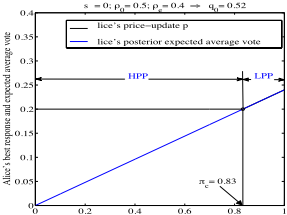
Figure 2 shows Alice's equilibrium report in a LMSR market and her expected market outcome vs. ⇡, for sA = 0 and fixed ⇢0↪ ⇢e (hence, a fixed q0). Note the HPP and LPP regions to the left and right of the cross-over probability, where Alice's price-report (the dashed curve) is distinct from and coincides with her expectation of the average vote (the continuous curve) respectively. The corresponding plots for the other two MSRs are qualitatively similar.
4 Discussion
Our model is stylized, but the framework and methodology can be applied to more complex scenarios. Below, we sketch two specific lines of generalization.
Additional outcome-deciders who do not trade: Consider a scenario in which Alice and Bob are the only traders but jointly decide less than 100% of the outcome, say, v = vA+vB+Pni=1 vi n+2 , where ¶vi♦ni=1 are the votes (and also the private signals) of n non-strategic agents. To solve for equilibria, we now need, in addition to Bob's non-participation probability ⇡ and Alice's posterior belief about others' signals given sA, Bob's posterior belief given sB and Alice's trading action; but we can use the same methodology as in Alice's posterior probability of Bob's signal being 0 (q 0 )
0.4
0.35
0.3
0.25
0.2
0.15
0.1
0.05
0
0
0.2
Probability (/) of Bob not participating in LMSRïmediated prediction market
Figure 2: Crossover from HPP to LPP equilibria regions for LMSR over 0 < ⇡ < 1 for a particular instantiation of the signal structure described in Section 3.2.
Section 3 to show that the PBE is still of two types (with some additional characteristics) depending on model parameters. For example, if all agents receive independent and identically distributed signals conditional on the type of the underlying entity, and the signal structure is such that vA = 0 if and only if sA = 0 (as in Section 3.2), then the main deviation from the analysis in Section 3 is that Bob's thresholds pL and pH now become functions of sB 2 ¶0↪ 1♦ so that each has two possible values. For a low enough ⇡, Alice's best response is to set pA at an uninformative value (pLsB=0 , pLsB=1 , pHsB=0 , or pHsB=1 ) but now STRATEGIC Bob decides whether or not to "agree with" Alice depending on sB, hence this equilibrium reveals Bob's signal; for a high enough ⇡, pA coincides with Alice's expected outcome but now her action fully determines STRATEGIC Bob's action, so Bob's signal cannot be inferred from his action, as in the two-player game; in either case, STRATEGIC Bob moves the price to his posterior expectation of v, which is no longer in ¶0↪ 1♦.
s A = 0; l0 = 0.5; le = 0.1 q 0 = 0.82 Alice's priceïupdate p A Alice's posterior expected average vote LPP HPP sign (as long as these successors are not outcome-deciders). The game becomes more complex for Alice when there are intermediate traders between Alice and Bob, but we believe that our model can serve as a foundation for analyzing this extension as well.
5 Conclusion
0.4 0.6 0.8 1 /c = 0.96 This paper is a first step in exploring the crucial incentive issues that have the potential to derail the effectiveness of prediction markets for various forecasting tasks. We have introduced a new formal model for studying the incentives for and the impact of manipulation in prediction markets whose participants can affect the outcome by taking actions external to the market but there is some uncertainty about the market participation of some outcome-deciders. We have characterized the equilibria of the induced game, discussed their properties, and outlined important extensions. Interesting avenues for future work include generalizing our results to markets with other price-setting mechanisms, richer signal structures, outcome functions other than the mean vote (such as nonlinear and / or noisy functions of the agents' second-stage actions), and agents who also strategically pick the time-points at which they trade.
Acknowledgments
We would like to thank Yiling Chen for helpful discussions. We are grateful for support from NSF IIS awards 1414452 and 1527037.
@inproceedings{ijcai2016p30,
  title     = {Trading on a Rigged Game: Outcome Manipulation in Prediction Markets},
  author    = {Chakraborty, Mithun and Das, Sanmay},
  booktitle = {Proceedings of the Twenty-Fifth International Joint Conference on
               Artificial Intelligence, {IJCAI-16}},
  publisher = {AAAI Press / International Joint Conferences on Artificial Intelligence},
  editor    = {Subbarao Kambhampati},
  pages     = {158--163},
  year      = {2016},
  month     = {7},
  url       = {https://ijcai.org/proceedings/2016/30},
}
TY - CPAPER TI - Trading on a Rigged Game: Outcome Manipulation in Prediction Markets AU - Chakraborty, Mithun AU - Das, Sanmay T2 - Proceedings of the Twenty-Fifth International Joint Conference on Artificial Intelligence, IJCAI-16 PB - AAAI Press / International Joint Conferences on Artificial Intelligence PY - 2016 SP - 158 EP - 163 UR - https://ijcai.org/proceedings/2016/30 ER -Copied
Machine-readable versions of this paper, for tools and AI agents:





