Using Message-Passing DCOP Algorithms to Solve Energy-Efficient Smart Environment Configuration Problems

1 Introduction

The rise of cheap and reliable technologies in the fields of Ambient Computing fosters the development of applications for smart environments, like smart homes. Such environments are equipped with devices with limited capabilities -e.g. wireless link with 250 kbps throughput, and microcontrollers with just a few KBytes of RAM- connected to a Home Area Network (HAN). These devices are used to provide services and make inhabitants live more comfortable. In addition to user preferences, global goals can be defined and applied to all scenes, to embody some global qualities that the system should have. Energy efficiency is an example of such a quality, where the system should always try to achieve the behavior requested by the user in the most energy efficient manner. However, developing such applications and coordinating such devices are still key research challenges for AI.

The introduction and the adoption of such smart environments could greatly gain by putting more "smart" into the objects and their infrastructure. Commercial solutions (e.g. from [Orange, 2016], [ARCHOS, 2016] or [Samsung, 2016]) have several major weaknesses. First, they require the user to define scenes he wants to be implemented by specifying conditions on the state of some sensors, and consecutive actions on the actuator devices (e.g. light bulbs or shutter locks). Even, he is asked to explicitly reference, one by one, every

Fano Ramparany

Orange Labs fano.ramparany@orange.com

object used in the scenario, which will prove difficult with a growing number of objects and when shifting from smart home to smart building scenarios. Second, when some devices are out-of-order or newly plugged to the building some user-defined rules may become inadequate, and the user has to manually update/add rules to take these changes into account. Finally, current solutions are lacking robustness and resilience. Solutions mainly rely on a mixed cloud and gateway infrastructure to control and monitor the system. Typically a physical home automation box hosts the building behavior and relies on proprietary cloud services to configure the devices. If this box is faulty, or internet connection is broken, the system will no more implement the specified behaviors (at best in a degraded mode). To overcome these limitations, one can make the devices interact seamlessly in the home and provide services without requiring the user to setup complex configurations to express his preferences. Objects should arrange among themselves and decide autonomously the best way to realize the requested behavior, without human intervention, based on the definition of rules that does not explicitly refer to specific equipments.

We address this spontaneous configuration problem using the distributed constraint optimization framework (DCOP), where devices are part of a multiagent system whose task is to maximize adequacy to user's requirements while meeting non-functional requirements on energy efficiency. We expound some background on DCOP in Section 2. The model for smart environment configuration problem (SECP) is detailed in Section 3, and translated into a DCOP in Section 4. Section 5 discusses how to deploy the factor graph resulting from the DCOP formalization in the physical devices. Section 6 presents results and analyses of experiments on realistic simulated smart home scenarios, as to benchmark different algorithms to solve SECP. Finally, we conclude this paper with some perspectives in Section 7.

2 Background and RelatedWorks

This section expounds the DCOP framework and some related algorithms from the literature are discussed, especially concerning their applicability to smart environment settings.

2.1 Distributed Constraint Optimization

One way to model the coordination problem between smart objects is to formalize the problem as a DCOP.

Definition 1 (DCOP) A discrete Distributed Constraint Optimization Problem (or DCOP) is a tuple hA↪X↪D↪ C↪ θi, where: A = ¶a1↪ ▷ ▷ ▷ ↪ a♣A♣♦ is a set of agents; X = ¶x1↪ ▷ ▷ ▷ ↪ xn♦ are variables owned by the agents; D = ¶Dx1 ↪ ▷ ▷ ▷ ↪Dxn ♦ is a set of finite domains, such that variable xi takes values in Dxi = ¶v1↪ ▷ ▷ ▷ ↪ vk♦; C = ¶c1↪ ▷ ▷ ▷ ↪ cm♦ is a set of soft constraints, where each ci defines a cost 2 R [ ¶1♦ for each combination of assignments to a subset of variables (a constraint is initially known only to the agents involved); θ : X ! A is a function mapping variables to their associated agent. A solution to the DCOP is an assignment to all variables that minimizes Pi ci.

A large literature exists on solution methods for DCOPs, which fall into two categories:(i) complete algorithms like ADOPT and its extensions [Modi et al., 2005], or inference algorithms like DPOP [Petcu and Faltings, 2005] or ActionGDL [Vinyals et al., 2010], are optimal, but mainly suffer from expensive memory (e.g. exponential for DPOP) or communication (e.g. exponential for ADOPT) load -which we may not be able to afford in a constrained infrastructure like our smart environment setting; (ii) approximate algorithms like Max-Sum [Farinelli et al., 2008] or MGM [Maheswaran et al., 2004] are usually faster with a limited memory print and communication load, but losing optimality in some settings. Yet, suboptimality may suffice especially when it comes to human interpretation and comfort. Both categories mainly exploit the fact that an agent's utility (or constraint's cost) depends only on a subset of other agents' decision variables, and that the global utility function (or cost function) is a sum of each agent's utility (constraint's cost). In the following, we will focus on two such inference algorithms.

DPOP. The distributed pseudo-tree optimization procedure (DPOP) is an optimal method implementing dynamic programming in a distributed way [Petcu and Faltings, 2005]. DPOP runs three phases. (1) It builds a depth-first search (DFS) tree that overlays the constraint network. This pseudotree, made of parent links and pseudo-parent links (when loops appear in the constraint graph) is used by agents owning variables to interact during the next phases. (2) Once the DFS tree is build, cost messages are sent by the leafs and propagate from children to parent up to the root. A cost message, assessed by joining all the messages received from children, is a relation associating a cost to every possible assignment of the variables in the agent's separator, i.e. the minimal set of ancestors whose removal completely disconnect the subtree rooted at this agent to the rest of the problem. (3) Once the root has received the cost messages from its children, it assesses the aggregated costs of the whole problem and then it decides the best assignment for its variables. Finally, it broadcasts this assignment in a value message to its children, who assess their best assignments and send them down the tree. DPOP returns an optimal assignment, with only a linear number of messages. Many DPOP extensions and other exact algorithms work in a similar way [Vinyals et al., 2010].

Max-Sum. There exists another class of algorithms, falling under the framework of the generalized distributive law [Aji and McEliece, 2000], that can be used to obtain good approximate solutions. Among them, Max-Sum is of particular interest in our case. It operates on a factor graph (FG): an undirected bipartite graph in which vertices represent variables and constraints (called factors) and edges link constraints to the variables in their scope. Messages will flow from factors to variables, and vice versa and are only associating costs to values of the recipient. A factor fm assesses the message Rm!n to a variable xn by adding its own cost cm to the costs received from all the variables connected to it, except xn, and choosing the best cost for a value of xn when several alternatives exists for obtaining this value. In return, a variable xn assesses a message Qn!m to factor fm by only adding messages received from connected factors except the factor fm. When a factor or a variable computes twice the same message for the same recipient, it stops propagation. The process ends at convergence or when a time limit is reached. MaxSum is complete for tree-shaped constraints graphs, suboptimal for loopy graphs where it may not converge at all. But it has been shown to compute better quality solutions than the approximate class with acceptable computation compared to representative complete algorithms [Farinelli et al., 2008]. Though, a bounded version of Max-Sum, that is able to efficiently compute solutions with a guaranteed approximation ratio, has been proposed in [Rogers et al., 2011].

2.2 DCOP for Ambient Intelligence Scenarios

As far as an ambient intelligence coordination problem is modeled as a DCOP -which is not always straightforwardthe aforementioned techniques can be used for finding the optimal configuration. Approaches exist to model such coordination problems as dynamic CSP [Degeler and Lazovik, 2013]. However, their approach is not distributed among devices. To the best of our knowledge, few past works have focused on the use of DCOPs in ambient environment settings, except [Pecora and Cesta, 2007], which uses a variant of ADOPT to coordinate ambient application services, and not devices themselves. Indeed, the proposed solution is not applicable to in-board implementation, due to ADOPT limitations. Closer works, not focused on smart environment, deploy DCOP algorithms on real constrained devices [Farinelli et al., 2008; Jain et al., 2009] for robotic or sensor coordination problems. In fact, ambient intelligence applications, while requiring efficient coordination of devices, may afford suboptimality: e.g., if an ambient system is asked to find the best configuration for emitting light at a desired level of 400 lumens and only achieve 380 lumens, it may not even be perceivable by the user, who may finally agree the actual service level. Message-passing inference approaches like MaxSum seem more relevant when it comes to deploy on-board [Farinelli et al., 2008]. But before discriminating optimal solutions, we propose to model a smart environment configuration problem to be solved by DCOP algorithms we will implement and evaluate, to support this hypothesis. In fact, depending on the DCOP model, the realistic number of devices, the nature of the constraints coming from the user requirements and the physical models (e.g. consumption laws of devices, influence of light bulbs on light level in a room), it is possible scalable complete algorithms, like DPOP, are efficient.

3 Smart Environment Configuration Problem

Here, we expound and illustrate the smart environment configuration problem we address in this paper.

3.1 Sample Scenario

We consider the following AmI scenario. Our system is made of several smart devices: light bulbs, roller shutters, a TV set, several luminosity sensors and a presence detector. Each such device is defined by (i) a unique identifier (e.g. its MAC address), (ii) its location (e.g. living room), (iii) a list of capabilities (e.g. emitting light or playing videos), (iv) a list of actions (e.g. setting power at 2Wh), (v) a consumption law associating an energy cost to each action. The user can use an application on a tablet to configure simple behaviors (or scenes), using the value of the sensors or the state of actuators as triggers for implementing smart home actions. For example, one could configure the system such that a luminosity level of 60 is reached in the living room whenever somebody is in this room. Note that the user does not need to specify which lamp must be used: the system autonomously decides the best way to achieve this target, by opening the shutter, dimming the lamp and maybe even switching the TV on if no other source of light is available. This also means that light bulbs may be added or removed and they will be automatically integrated into the system. We want our system to choose the most energy-saving configuration for a given scene.

Example 1 (Scene specification) Rule (1) defines a scene where the light level of the living room should be set at 60 lumens whenever someone is present in the room:

Rule (2) refines rule (1) by triggering only when the light level is less than 60 lumens and closing the shutter of the living room as an additional action:

This problem is close to what is proposed in [Degeler and Lazovik, 2013], a rule-based dynamic constraint satisfaction approach, but our requirements imply embedding the coordination protocol within devices. Alternatively to satisfaction, this configuration problem can be seen as an optimization problem with values to assign to actuators (e.g. a light bulb is assigned a power) and user's target values (e.g. the light level in living room is 60 lumens), whilst maximizing the adequacy to user-defined scenes and minimizing the overall energy consumption.

3.2 ProblemDefinition

Let A be the set of available actuators. We note ⌫(A) the set of variables stating the values of actuators i 2 A (e.g. the power assigned to a bulb). We use xi to refer to a possible state of xi 2 ⌫(A), that is xi 2 Dxi (domain of xi). Each actuator i has a cost to be activated, noted ci : Dxi ! R. This cost can be directly derived from the consumption law of each device (e.g. mapping a cost in euro to each action). We note C = ¶ci♣i 2 A♦. Among the possible values, every actuator i has a possible "switched off" state value, noted 0 2 Dxi , with an associated cost (most probably 0).

Let S be the set of available sensors, and ⌫(S) the set of variables encapsulating their states. We note s` 2 Ds` the current state of sensor ` 2 S. Sensor values are not controllable by the system: they are read-only values.

Let R be the set of user-defined scene rules. Each scene k is specified as a condition-action rule expressed using the set of available devices (actuators and sensors) and capabilities. The condition part of a scene is specified as a conjunction of boolean expressions using state of actuators (e.g. power of light bulb #1 is greater than 2Wh) or state of sensors (e.g. someone is present in the living room) and binary predicates (e.g. >, <, =). The action part of scenes defines target values for either (i) some direct actions on actuators (e.g. power of light bulb #1) or (ii) indirect actions (or corresponding to users' goals) on more abstract concepts (e.g. light level in living room) -both are called scene action variables.

These scene action variables are therefore either (i) some xi 2 ⌫(A) or (ii) other values constrained by values assigned to some actuators (e.g. the light level of living room depends on the power assigned to the two light bulbs in this room). We note yj 2 ⌫(Φ) the state of such an indirect scene action j (e.g. the current level of light in a room). We note xki (resp. yk j ) the target value defined by the user for the scene action variable xi (resp. yj) in the rule k. We use yj to refer to a possible state of yj, that is yj 2 Dyj (domain of yj). Obviously, xki 2 Dxi and yk j 2 Dyj for all i, j and k. Note that a scene action variable can be used in several rules, but that a rule can only specify a unique target value for the scene action variable.

A scene rule can be either active or inactive depending on the state of devices appearing in the condition part of the rule. Each active scene has also a utility to be implemented, noted uk : Qs2σ(uk) Ds ! R, with σ(uk) ✓ ⌫(A) [ ⌫(Φ) being the scope of the rule (the subset of variables used in the rule). The more the states of the scene action variables (from ⌫(A) and ⌫(Φ)) are close to the user's target values for this scene, the higher the utility. Moreover, if the condition to activate the rule (from ⌫(A) and ⌫(S)) are not met, the utility should be neutral, i.e. equals to 0. We can therefore consider uk's to be functions of the distance between the states of the scene action variables xi's (resp. yj's) and the target values xki (resp. yk j ). We note U = ¶uk♣k 2 R♦.

Example 2 (Scene rule utility) Let us consider rule (1), where s1 is the value of the presence sensor. Here a possible utility function, which is the negated distance between the current value of y1 and the target value y1 1 = 60 defined in rule (1):

Here a possible utility function for rule (2), where s2 is the sensed light level and x3 is the level of the shutter:

Each scene action variable yj depends physically on the values of several actuators. We note the model of this dependency φj : Q&2σ(φj) D& ! Dyj , where σ(φj) ✓ ⌫(A) is the scope of the model, i.e. the set of variables influencing yj. Let φj = ♣σ(φj)♣ the arity of φj, and Φ = ¶φj♦ be the set of all physical models between actuators and user-defined values. In a more general form, a physical dependency model links a set of objects -with a given capability (e.g. emitting light, like a bulb or a TV set), in a given location (e.g. living room)- to a physical value (e.g. light level) that can be measured by some sensor (e.g. light sensor).

Example 3 (Physical model) We can consider that the level of light y1 in a room depends on the total power of installed "light-emitting" devices installed in the room, i.e. bulbs x1 and x2, and a TV set x3:

Weights assigned to each xi is related to the luminous efficacy of each device [Stimson, 1974].

Given all the previous concepts and notations, we define SECP as follows:

Definition 2 (SECP) Given a set of actuators A (and their related costs ci 2 C), a set of sensors S, a set of scene rules R (and their related utility functions in uk 2 U), and a set of physical dependency models Φ, the Smart Environment Configuration Problem (or SECP) hA↪ C↪ S↪ R↪ U↪ Φi amounts to finding the configuration of actuators that maximizes the utility of the user-defined rules, whilst minimizing the global energy consumption and fulfilling the physical dependencies.

4 Formulation of SECP as a DCOP

SECP can be straightforwardly mapped to a multi-objective optimization problem:

The multi-criteria problem (3) can be formulated as a mono-objective problem by aggregating the two objectives, provided that the ranges of uk's and ci's are normalized or prioritized (using weights !u↪ !c > 0):

Hard constraints corresponding to physical dependencies are encoded as factors noted 'j , to translate (4) into a DCOP. We note Φ the corresponding set of 'j 's.

Using equation (5), SECP is then formulated as a DCOP hA↪X↪D↪ C↪ θi where: A is a set of smart devices; X = ⌫(A) [ ⌫(Φ); D = ¶Dxi ♣xi 2 ⌫(A)♦ [ ¶Dyj ♣yj 2 ⌫(Φ)♦; C = U [ C [ Φ; θ is a function that maps variables and constraints to smart devices; with the following objective:

Such a DCOP can be represented as a factor graph, noted G = hVx↪ Vf ↪ Ei, which is a generalization of classical constraint graphs [Farinelli et al., 2008]. For SECP, variable nodes are taken from Vx = ⌫(A) [ ⌫(Φ), connected through factors in Vf = U [ C [ Φ by applying the following rules: (i) each xi 2 ⌫(A) is a variable node, (ii) each xi 2 ⌫(A) is connected to a unary factor ci specifying its cost, (iii) each yj 2 ⌫(Φ) is a variable node, (iv) each yj and all xi 2 ⌫(A) in the scope of a physical dependency model φj are connected to a factor 'j, (v) each scene rule k 2 R is represented by a utility factor uk -which is a function of the distance to the target values xki 's and yk j 's and the current values of all variables in σ(uk)- connected to all the xi 2 σ(uk) and yj 2 σ(uk). As to explicit the information coming from sensors' state that may trigger rules, we add read-only variables for each sensor state s` 2 S, like in [Pecora and Cesta, 2007]. Formally, each such a read-only variable can be considered as a variable-factor pair hs`↪ f`i, where:

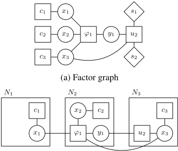
Example 4 (Factor graph) Fig. 1a represents a factor graph for rule (2), where x1 is the state of the light bulb #1; x2 is the state of the light bulb #2; x3 is the state of the shutter; y1 is the light level in lumens; c1, c2, c3 are costs to activate actuators; u2 is the factor representing the scene rule and defining the utility depending on a target value y2 1 for variable y1; y1 is the variable representing the theoretical light level in lumen; '1 is the physical dependency model between the light level and the state of actuators; s1 and s2 are read-only variable nodes, represented as dotted diamonds.

5 SECP Deployment and Solving

In our setting, connected objects cooperate autonomously to reach the user-specified goals. Now that we have modeled this cooperation as a DCOP, we map the corresponding FG into the available physical devices, and explain how it is deployed within the available nodes/agents before running a message-passing algorithm like Max-Sum or DPOP.

Our devices are assumed to be resource constrained and the communication link between them is implemented with a low power network with limited throughput (typically 250 kps). Devices with only a sensing role are usually powered on battery and run as sleepy nodes, meaning that they switch off their communication interface most of the time in order to save energy and only turn it on when they want to emit a new value. As a result, these nodes cannot be reached most of the time and are not good candidates to host the computations needed for the variables and factors in our DCOP. On the

(b) Sample distribution

Figure 1: Factor graph (1a) and a possible distribution (1b) on 3 agents (N1, N2 and N3) for the SECP for rule (2)

other hand, actuators, and especially light sources, are usually connected to the main power line and always reachable. So, our FG is only hosted on the actuator devices, called agents. Agent with actuator i is denoted Ni and the set of agents corresponds to A.

The distribution of a DCOP is usually given by a function θ which maps each variable in the DCOP to an agent. Here, as we use a FG model, and because in Max-Sum factors correspond to computation to perform, we also map factors to agents. Formally, defining an optimal mapping is an optimization problem by itself, namely graph partitioning, which typically falls under the category of NP-hard problems [Bichot and Siarry, 2011]. Since this paper does not focus on this specific problem, we only provide here a heuristic mapping, defined as follows.

xi variables and ci factors are naturally hosted on agent Ni, which they represents. Variables and factors yj, 'j and uk do not map directly to any physical devices and must be distributed on existing agents. Each pair hyj↪ 'ji is hosted on a agent Ni with i chosen such that xi 2 σ(φj), meaning that xi is one of the variables influencing yj. Similarly the factor uk is hosted on a agent Ni such that xi 2 σ(uk). Intuitively this means that the factor representing a rule is always hosted on a agent affected by this rule. This distribution reduces the amount and size of messages between agents when solving the DCOP. As to ensure a balanced computation load, yj's, 'j's and uk are fairly distributed among the candidate agents. This gives us the following definition for the mapping function:

Fig. 1b represents a possible distribution of computation with each agent denoted with a dotted rectangle, for the FG presented in Fig. 1a.

The deployment is performed once the user has defined the rules. This operation is performed on a smartphone (or a tablet), which is only part of the system during this phase: once the system is configured the smartphone is switched off and the devices operate autonomously. To deploy the DCOP, the program on the smartphone must perform two tasks. First it compiles the uk factors. As a user-defined rule k is embodied in the factor uk, which encodes the target values xki and yk j (for all xi and yj in σ(uk)) defined in the rule k, this factor must be re-compiled whenever the rule is modified. Second, it must assign each element v of the FG to an agent using the mapping function θ. Once the FG of the SECP specified by the user deployed, the smart devices are configured to implement a message-passing protocol, like DPOP or Max-Sum, to solve this specific instance. From then, the system is autonomous and self-configures without user intervention. For instance, if a device is newly introduced, systems finds another alternative configuration that meets user's requirements, by only running the same protocol.

6 Experiments on Simulated Environments

In order to analyze the applicability of DCOP solvers to SECP, we implement and evaluate DPOP and Max-Sum on randomly generated instances. We consider here a realistic smart house with actuators (light bulbs), physical models and user-defined scene rules. Each actuator/light is associated with an efficiency factor, which defines a cost function as a linear function of the emitted luminosity. Physical dependency models are weighted sums of the luminosity levels emitted by the light bulbs in its scope and yield the theoretical resulting luminosity in a given place as an indirect scene action variable. Finally, rules assign target values to one or several scene action variables (actuators and models). Variables, models and rules are randomly connected and we only consider active rules, which have an actual influence on the problem. The resulting SECP is deployed as described in Section 5. As physical models map to different rooms and spaces in the house, which might be independent one from the other, the corresponding house-level SECP can generally be divided into several independent subsets that can be solved in parallel. As this would distort results, all our experiments are made on indivisible SECPs, which can be mapped to connected FGs. For each problem size (same number of rules, models and actuators), 30 instances are generated and solved. The average of the results are plotted.

In our first experiment, SECP are generated with 10 actuators, 5 rules and a growing number of models (from 1 to 20). As the corresponding FG are connected, each rule constrains a growing number of models. Figure 2(a) shows the total number of exchanged messages (log scale). Clearly, MaxSum generates more messages before converging. However Figure 2(b), where total message size is given as the number of transmitted variable values and costs (encoded as floats), shows that DPOP generates a larger network load for complex problems. Even while generating less messages than Max-Sum, DPOP is still more communication-extensive than Max-Sum. Moreover Max-Sum is remarkably stable and its total message size grows slowly with the number of models.

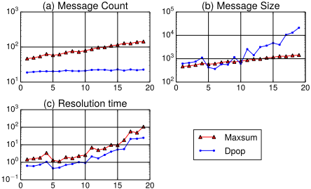
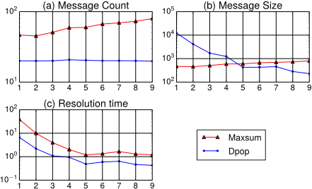
Figure 2(c) shows the time (in seconds) taken by Max-Sum and DPOP to solve the SECP instances. Surprisingly, even if Max-Sum is a approximate algorithm, DPOP solves the instance faster than Max-Sum but the difference is stable, which means it might be implementation-dependent.

In our second experiment, SECP are generated with 10 actuators, 5 models and a growing number of rules (from 1 to 10). Figures 3(a) and 3(b) show respectively the total number and size of messages exchanged ; as before DPOP generates less messages but can produce a higher network load for complex problems. With both algorithm, we see that SECP with more rules are simpler ; this is due to the decrease in the average arity of the rules and models as the number of rules increases, as we only consider SECPs with a connected FG.

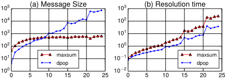
In our third experiment, we generate a very large number of connected SECP with a random number of actuators, models and rules. Figure 4(a) and 4(b) shows respectively the size of messages exchanged and the resolution time plotted against the number of cycles (i.e. cardinality of the cycle basis) in the corresponding FG. Clearly, the complexity of the SECP depends on the number of cycles in the graph but Max-Sum manage to keep a remarkably stable message size independently of the problem's complexity.

We use DPOP as a reference optimal cost to evaluate the quality of the solutions provided by Max-Sum. In 99.5% of our test cases our implementation of Max-Sum is optimal, despite the high cyclicity of the SECPs the global cost of the solution it produces is the same than the cost of the optimal solution produced by DPOP. When several equivalent symmetric solutions exist, Max-Sum might break an hard constraint corresponding to a physical model. In order to break ties we introduce random noise to the actuator costs. In our experiments, the remaining 0.5% of non-optimal solutions correspond to cases where this approach fails to break ties.

7 Conclusions and Perspectives

We have presented a model for coordinating connected devices in a smart environment. Devices operate themselves the configuration process, without supervision. The model makes use of physical relations between objects as to prevent the user to explicitly specify the role of each object, easing the definition of rules and the introduction of new devices at runtime. We propose to use message-passing methods, like DPOP and Max-Sum, to implement the coordination protocol. From our experiments on a simulated smart home scenario, Max-Sum is best suited for the constrained devices commonly used in smart environment and our SECP model is a viable approach for autonomous coordination among these devices.

There are several paths to future research. First, we assumed that physical models linking devices to sensed measured are a priori known. However, physical dependencies may strongly depend on the positioning of devices. Therefore, we will investigate inexpensive methods for learning this models from sensed data, like simple polynomial regression, that could be embedded into devices. Second, we have directly used on-the-shelf methods without adapting them to the specific case of SECP. But, due to the specification of the physical factors (e.g. weighted sum) and the loopy nature of the graph, we will investigate a dedicated algebra for messages, to make them more compact and faster to assess. Third, instead of handling multi-objectiveness using penalization, we wish to cast our SECP into the multi-objective DCOP framework (MO-DCOP) [Matsui et al., 2012]. Finally, as to provide openness and adaptiveness, we need to consider the resilience of the proposed approach, by providing mechanisms to handle device (dis)appearance and using redundancy in the factor graph deployment, without impacting the performances, like proposed in a centralized way in [Degeler and Lazovik, 2013].