Towards a White Box Approach to Automated Algorithm Design

1 Introduction

There are many ways to solve a given problem. Therefore, when faced with a problem, we must choose an algorithm to solve it (the algorithm selection problem [Rice, 1976]). In general, the best algorithm depends on the context in which it is used (e.g. problem instance, execution environment, etc.). Furthermore, these methods often have many parameters/components that require appropriate tuning and configuration to achieve satisfactory performance (the algorithm configuration problem [Hutter et al., 2009]). To date, algorithms for many real-world problems are most commonly designed using a manual, ad-hoc, trial & error approach, making algorithm design a tedious, time-consuming and costly process, often leading to mediocre results.

Recently, Programming by Optimization (PbO) [Hoos, 2012] has been proposed as an alternative design paradigm in which difficult choices are deliberately left open at design time, resulting in a rich and potentially large design space, rather than a single algorithm. Subsequently, optimization methods are applied to automatically generate the best algorithm instance for a specific use-case. PbO distinguishes itself from Genetic Programming [Koza, 1992] in that it attempts to maximally utilize expert knowledge to prune the design space, which typically only consists of algorithms solving the problem considered correctly. To date, optimizers of choice for PbO are algorithm configuration methods. Algorithm configurators search a space of configurations to find one that optimizes the performance of an algorithm over a given set of training instances (inputs). Configurators such as ParamILS [Hutter et al., 2009], iRace [L´opez-Ib´anez et al., 2011] and GGA [Ans´otegui et al., 2009] are able to configure hundreds of parameters and represent the state-of-the-art. These methods require very little expert knowledge to use them, however, they are limited by the fact that they return a single configuration to be used on any input encountered in practice. As such, they don't solve the algorithm selection problem, making them susceptible to overfitting and no-freelunch theorems [Wolpert and Macready, 1997]. Therefore, context-aware configurators have been proposed that solve both algorithm configuration and selection problems simultaneously by learning a configuration selection portfolio (e.g. Hydra [Xu et al., 2010] and ISAC [Kadioglu et al., 2010]).

In this paper, we address another weakness of contemporary algorithm configurators w.r.t. solving the Algorithm Design Problem (ADP): They consider algorithm performance as a black box, where a cost function maps a configuration and input to a real cost-value. They do not exploit the fact that this mapping is a consequence of algorithm execution, i.e. design decisions affect the execution path for an input in a particular way, which in turn relates to execution cost. To this purpose, we propose an alternative white box approach to the ADP. In Section 2 we reformulate the ADP as a Markov Decision Problem, capturing the intrinsic relationships between design decisions and their contribution to overall algorithm performance, including an explicit notion of context. Subsequently, we discuss possible solution approaches in Section 3. In Section 4 we discuss how white box information could be used to speed up the meta-optimization process and improve the quality of the resulting design. In Section 5 we describe a concrete implementation of a white box optimizer as a Proof of Concept, and use it to illustrate some of these benefits experimentally in Section 6. Finally, we discuss related research in Section 7 and conclude in Section 8.

2 The AlgorithmDesign Problem (ADP)

2.1 Black Box Formulation

Let ∆ be the set of design choices,  a function mapping each design choice to a set of alternative decisions and C = ¶c♣c(dc) 2 (dc)↪ 8dc 2 ∆♦ the set of possible configurations. The traditional Black Box Algorithm Design Problem can be formulated as follows: Given a probability distribution D over the set of possible inputs X and an algorithm evaluation function f : X ⇥ C ! R, find a configuration c⇤ satisfying c⇤ = argmaxc0 Ex⇠Df(x↪ c0 ), i.e. maximizing the expected evaluation function value w.r.t. D.

2.2 White Box Formulation

In this section, we propose an alternative (white box) formulation, exposing the internal structure of f. Here, we consider algorithm design as a sequential decision process. Informally, we start executing an algorithm with open design choices. As long as the next instruction does not depend on the decision made for any of these, we simply continue execution. When it does, a choice point is reached, and a design decision must be made in order to continue execution. This process continues until termination. In what follows, we formalize this process. We first extend the Turing Machine (TM) [Turing, 1936] to include open design choices, their respective domains, and a notion of the desirability of an execution. Starting from the definition of a TM as a 7-tuple hQ↪ Γ↪ B↪ ⌃↪ δ↪ q0↪ F i given in [Hopcroft, 1979, p. 319], we define an Algorithm Design Process as a 10-tuple: TM adp = hQ↪ Γ↪ B↪ ⌃↪ ∆↪ ↪ δ0 ↪ ⇢↪ q0↪ F i:

• Q is a finite, non-empty set of states.

Γ is a finite, non-empty set of tape alphabet symbols.

B is the blank symbol.

• ⌃ ✓ Γ ∩ ¶B♦ is the set of input symbols.

∆ is the set of choice points or design choices.

•  is the domain function ∆! 2Q⇥Γ⇥¶right↪left♦ .

δ0 is the open transition function

⇢ is the reward function (Q∩F)⇥Γ!R. Representing the contribution of a transition to overall performance (f).

q0 2 Q is the start state.

Let ↵zbβ be an Instantaneous Description (ID) of TMadp, with current state or choice point z, tape content ↵bβ, head pointing at b. Here, ↵ and β denote a prefix and suffix of zero, one or more tape symbols. Let ↵zβ ` id 0 represent a single move of TMadp. If z 2 ∆, an agent selects the next move a 2 (z) the TM will perform (denoted by `a ), otherwise TMadp is simulated as an ordinary TM. Finally, id `⇤ id 0 indicates that simulating TMadp from id for zero, one or more moves results in id 0 for some choices of the agent.

F ✓ Q is the set of final states.

Note that TMadp can be seen as a Non-deterministic TM having rewards associated with its transitions. The objective of an agent in the ADP is to determine these nondeterministic transitions as to maximize the reward it accumulates: Pni=1 ⇢(qi↪ bi) where qi and bi are the ith of the n states and tape symbols read by TMadp, before halting. In what follows we assume any simulation of TMadp will eventually halt (independent of the agent's decisions).

We now rephrase TM adp as a deterministic Markov Decision Process (MDP) [Bellman, 1957]: MDPadp = hS↪ A↪ T↪ Ri:

A = Ss2S As is the set of actions, where A↵zβ = (z) if z 2 ∆, As = ¶anoop♦ otherwise.

S = ¶↵zβ ♣ 9x 2 X : q0x `⇤ ↵zβ↪ z 2 (¶q0♦ [∆)♦ [ ¶⌧♦ is the set of states, where ⌧ is the terminal state.

T : S ⇥As ! S is the transition function. Let next(id) be the ID resulting from simulating TMadp starting from id until it halts or a choice point is reached.

T (⌧↪ anoop) = ⌧▷

R : S ⇥As !R is the reward function.

R(s↪ a) = Pni=1 ⇢(qi↪ bi) where qi and bi are the ith of the n states and tape symbols read by TM adp while performing the simulation for T (s↪ a).

In state ↵zβ the agent is faced with design choice z. We will refer to the combination of tape content (↵β) and head position as the context in which this design choice is to be made. A solution to an MDP is a policy ⇡ : S ! A, corresponding to an execution context dependent configuration. For a given policy, an MDP reduces to a Markov Chain and the formulation for TMadp can be reduced to that of an ordinary Turing Machine, i.e. the algorithm corresponding to this configuration. The white box ADP as such reduces to finding a policy ⇡⇤ satisfying

V⇡ is called the value function and gives the total reward that will be received following a given policy ⇡ from state s. In particular V⇡(q0x) = f(x↪ ⇡)↪ 8x 2 X. Since ⇡⇤ optimizes V for any state, it obtains optimal performance on every input and therefore any distribution D.

Remark that MDPadp is deterministic. Algorithms are never truly non-deterministic. Rather, stochasticity is a consequence of pseudo-random numbers computed deterministically from a given seed value, which is part of the input. Alternatively, assuming the seed value is drawn from a stationary distribution, we can reformulate transitions in MDPadp to be stochastic: replacing T (s↪ a) by P (s↪ a↪ s0 ), yielding the probability that taking action a in state s leads to state s0 .

3 Solving the AlgorithmDesign Problem

Assuming S is finite, equation 1 (and its stochastic variant) can be solved using dynamic programming. Commonly used methods include Value and Policy iteration [Bellman, 1957; Howard, 1960], and their extensions. Note that these approaches require P and R to be known explicitly. However, in our formulation, P and R are consequences of execution (TM simulation). In some cases, P and R can be derived from the source code. Otherwise, we can estimate P and R based on repeated simulation and compute ⇡⇤ afterwards using dynamic programming. Alternatively, model-free Reinforcement Learning (RL) techniques can be used to learn ⇡⇤ online, directly from the rewards and transitions observed during simulation [Sutton and Barto, 1998].

A complicating factor in solving real-world white box ADPs in practice is the fact that the context space (i.e. all possible memory states of the program) can be extremely large. Fortunately, the best decision will typically depend on only a subset of all context information. Furthermore, it is possible to exploit an arbitrary subset of observable/relevant features [Kaelbling et al., 1998]. In addition, we can focus on relevant states, i.e. those that actually occur in practice (e.g. using prioritized sweeping, on-policy RL). Finally, solving MDPs with large state-action spaces has been an active research area for several decades [Wiering and van Otterlo, 2012], resulting in various techniques (e.g. incorporating function approximation). Exploring these in context of the implementation of a concrete solver is subject of future research.

4 Benefits of aWhite Box Approach

In this section we discuss potential benefits of following a white box approach to the ADP. First we briefly clarify the relationship between the white box ADP formulated in Section 2.2 and the traditional black-box ADP described in Section 2.1. These are not equivalent, rather the latter can be seen as a formulation of the former as a problem that can be solved using existing configurators. This formulation abstracts information that is naturally available in a PbO setting and restricts candidate designs to the set of static configurations. In Section 4.1 we describe how simulation-based solution techniques can exploit white box information to solve a given ADP faster. In Section 4.2 we discuss the benefit of considering adaptive designs as candidates in the ADP.

4.1 Speed upMeta-optimization

Black box evaluation of a configuration results in a single value (f), obtained after execution. White box evaluation on the other hand gives us a list of tuples (si↪ ai↪ ri), in chronological order, over the duration of the run, i.e. the state (choice point, context) si encountered, the action (decision) ai taken, and the corresponding reward ri received. Note that f can be deduced from this data (f = P ri).

Black box evaluation of a configuration on one input does not provide any information about the performance of other configurations, or performance on other inputs. Since runs using different configurations and inputs might have large parts of their execution in common, i.e. encounter similar states, white box information can be generalized across designs and inputs, improving data efficiency. This fact can be exploited to perform more informed sampling and reduce the estimation error in a stochastic setting, i.e. speed up the optimization process. E.g. Design decisions only affect execution after they are made, i.e. only rewards received after making a certain decision can be attributed it. As a consequence, data can be shared across configurations for as far as they make the same decision in the states encountered thus far. Also, often only a subset of choice points is encountered during a run, i.e. multiple configurations correspond to the same execution path. In Section 5.2 we describe PURS, an agent using this information to sample uniformly at random w.r.t. execution paths, rather than configurations. Remark that some black-box optimizers allow the user to specify dependencies between design choices. However, this is only possible if these are input independent and demands considerable expert knowledge. Also, methods attempting to profit from relations between design decisions do exist (e.g. SMAC [Hutter et al., 2011]). However, they do so by analyzing the cost function as a black-box, rather than by exploiting its internal structure.

Finally, black-box optimization typically requires many evaluations, which is problematic when these are expensive. Since white box information becomes available at runtime and states often repeat themselves within a single run, online learning (e.g. RL) can be used to evaluate multiple configurations over the course of a single execution. Which is for example useful to optimize parameters of a web-server.

4.2 Better/Adaptive Designs

Candidate solutions of the traditional black box ADP are configurations (∆ ! A). In our white box formulation, solutions take the form of execution context dependent configurations (Context ⇥ ∆ ! A). As a consequence, the white box ADP subsumes the algorithm selection problem. Rather than learning a configuration that is best on average, we learn the best configuration for each context (⇡⇤ ). Since ⇡⇤ is independent of the input distribution D, we can re-use white box information in settings where D might differ/change and can readily use any new experience to improve our policy (e.g. continuous improvement) without the risk of biasing our design.

Remark that a white box approach is not required to solve both algorithm configuration and selection problems simultaneously. Recently, black box solvers have been proposed (e.g. Hydra, ISAC) learning which configuration to use for a given input (X ⇥∆ ! A). However, the white box approach by nature considers the dynamic variant of the problem: "What configuration to use in a given execution context". As such, we're able to change our design decision dynamically, i.e. different decisions can be made in different execution contexts, even though the input is the same. In addition, black-box methods require a given set of (statically computed) problem features predictive for the performance of any particular configuration. The white box approach on the other hand, can use dynamic features of the resulting execution states. E.g. consider an algorithm taking the seed for a random generator as input (e.g. benchmark 2, Section 6.2). While computing relevant static features from a seed value is clearly troublesome, determining features of the resulting execution states is often trivial (e.g. the current iteration i).

Finally, since the white box ADP considers the superset of adaptive designs, it is potentially more difficult than its black box counter-part, depending on the extent we can exploit white box information to solve it. However, one could restrict the policy space and still exploit white box information to solve the resulting ADP more quickly.

5 AContext-oblivious White Box Optimizer

As explained in Section 3, implementing a (practical) general solver for the context-aware setting is challenging and subject of future research. In this section, we formulate and describe a solver for a "context-oblivious" variant of the ADP to demonstrate that our approach is practical nonetheless. In Section 6, we use this optimizer to illustrate some of the benefits of white box evaluation experimentally.

5.1 The Context-oblivious ADP (COADP)

In the COADP, decisions are made without using execution context information. In what follows, we show that the COADP can also be formulated as an MDP. Here, we further restrict our set of policies to those consistently making the same decision for a design choice during execution. Let C 0 = ¶c0 ♣c0 (z) 2 ((z) [ ¶✓♦)↪ 8z 2 ∆♦ be the set of partial configurations. A design choice z is said to be open in c0 if c0 (z) = ✓. Let next 0 (id↪ c0 ) be the ID resulting from simulating TMadp starting from id, choosing c0 (z)↪ 8z, until it halts or a design choice open in c0 is reached. Formally, next 0 (id↪ c0 ) = next(id) = ↵zβ if c0 (z) = ✓ and next 0 (id↪ c0 ) = next 0 (id 0 ↪ c0 ) with ↵zβ `c0 (z) id0 otherwise.

T co ((zx↪ c0 )↪ a) = s0 ▷ Let ↵zβ = next 0 (q0x↪ c0 ) and ↵zβ `a id 0 and ↵0 z0β0 = next 0 (id 0 ↪ c00 ) with c00 (z) = a and c00 (dc) = c0 (dc)↪ 8dc 2 ∆ ∩ ¶z♦. If z0 2 F: s0 = ⌧ , otherwise s0 = (z0x↪ c00 ).

Note that the resulting state transition graph is directed acyclic (with exception of the terminal state).

Remark that MDPcoadp actually corresponds to a set of independent MDPs, one for each input. As a consequence, this formulation doesn't allow us to generalize observations across inputs directly.

5.2 The Solver

We have implemented our optimizer as a standalone Java Library. 1 It solves the stochastic variant of the context-oblivious ADP (MDPcoadp) offline. It doesn't come close to exploiting the full potential laid out in Section 4. Rather, it serves as a Proof of Concept, demonstrating that it is relatively easy to implement and use a basic white box optimizer in practice.

Problem Specification

The programmer statically declares the design choices (∆) and their respective domains (). Users can define any domain they desire by implementing DesignChoice<T>. The generic type T allows the compiler to guarantee type safety. The library itself already provides some constructors for common domains (e.g. IntegerInRange, implementing DesignChoice<Integer>). Currently, the optimizer only supports discrete domains. When a decision is required for a design choice (choice point in δ0 ), a call to T getDecision(DesignChoice<T>) will return the decision for that choice. The feedback(Double) method is used to reward/penalize (⇢) the agent during execution, indicating the desirability of the current execution path. E.g. if f corresponds to "execution time", the feedback signal (R) corresponds to "the time elapsed between 2 choice points". For some f, assigning credit to parts of the execution might be difficult, in which case potential-based reward-shaping [Ng et al., 1999] can be used (without affecting ⇡⇤ ).

1 https://github.com/Steven-Adriaensen/White-box-ADP

Solution Approach

Our optimizer iteratively evaluates a given algorithm (with open design choices) on a given input (with variable seed). When an open design choice is encountered at runtime, it will query a given agent for a decision. Currently the following agents are supported:

• ÷ URS: Selects an alternative uniformly at random.
• ÷ PURS: Selects an alternative that was not yet selected uniformly at random, if any. Otherwise, an alternative a is selected proportional to the expected number of execution branches N(s↪ a) = Ps0 P(s↪ a↪ s0 )N(s0 ) with N(s) = Pa N(s↪ a) and N(f ) = 1.
• ÷ GR: Pure greedy, selects the alternative estimated to maximize the expected future reward.

When testing, we wish to use an agent that follows an optimal policy (i.e. GR). However, during the training phase the agent should explore alternative design decisions (e.g. (P)URS), i.e. guide the search.

During these evaluations, the following information about state transitions is recorded:

• ÷ n(s↪ a↪ s0 ): The number of times taking decision a in state s led to state s0 .
• ÷ r(s↪ a↪ s0 ): The average reward received after taking decision a in state s, before ending up in the next state s0 .

To reduce space requirements, these were only stored for the s↪ a↪ s0 encountered and assumed to be 0 otherwise. This information is used to approximate P co and R of MDPcoadp:

Finally, the optimizer assumes the best design, at any time, to be the policy ˜⇡⇤ solving^ MDPcoadp = hSco ↪A↪ ˜ P co ↪ ˜Ri. Here ^ MDPcoadp is solved using a bottom-up dynamic programming approach and ties are broken randomly. The idea is that multiple evaluations will allow us to accurately approximate the actual MDP and therefore its optimal policy.

Note that ^ MDPcoadp is a consistent estimator for MDPcoadp as long as each policy ⇡ has a positive chance of being explored. Our optimizer is therefore Probabilistically Approximately Correct [Valiant, 1984] as long as the agent used has this guarantee (e.g. (P)URS).

6 Experimental Illustrations

In this section, we illustrate some of the benefits of white box evaluation. To this purpose, we compare the performance of the implementation described in Section 5 to that of a similar black box implementation on two micro-benchmarks. These implementations differ in that the white box optimizer (WB) maintains transition data (n,r) and returns ˜⇡⇤ , while the black box optimizer (BB) maintains a c ! ¯ f(c) mapping and returns ˜ c⇤ = argmaxc0 ¯ f (c0 ).

Both optimizers perform Uniform Random Sampling. URS was chosen to keep things simple and illustrate the contribution of using white box information by itself. On some problems other features of state-of-the-art configurators (e.g. local search) might render white box benefits to some extent redundant. In general, white box evaluation is orthogonal to these more advanced sampling schemes and can be used to inform them (c.f. PURS for URS). Our experiments are by no means intended as a comparison of/to the state-of-the-art (WB nor BB are). The benchmarks have been selected to illustrate the benefits of our white box approach. We make no claims about their representativeness for real-world problems.

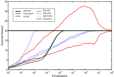
Figures 2 and 4 show the performance of the algorithm returned by each optimizer, after x algorithm evaluations, 2 averaged over 100 independent meta-optimization runs. Here we distinguish between the actual performance (full line) and the performance as estimated by the optimizer (dashed line).

6.1 Benchmark 1: Speed upMeta-optimization

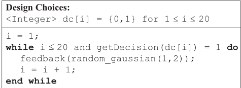
Figure 1 shows the code for benchmark 1. In this benchmark, we are to make up to 20 design decisions between 0 and 1, in a fixed order. As long as we choose 1, we receive a reward drawn from N(1↪ 2), otherwise execution terminates. While there are 220 different configurations, there are only 21 different execution paths, and ⇡⇤ (s) = 1↪ 8s.

Figure 2 compares our WB optimizer using the URS and PURS agents to the BB optimizer (BB-URS). We observe that each method overestimates the performance of its incumbent design. This schism is known as overconfidence (oc) [Birattari and Dorigo, 2004] and is caused by the fact that the maximum sample average is a biased estimator. Due to oc, an optimizer cannot distinguish bad from good designs, causing unreliable performance. BB-URS clearly exhibits most oc and performs the worst. It is only after about 1M evaluations that oc drops as configurations are re-evaluated. The WB optimizers have a much lower estimation error, as they are able to generalize across configurations. By reusing information obtained during the evaluation of similar policies, they improve their estimate of the performance of the best policy so far. Both URS methods take a long time, given there are only 21 execution paths. This is because, even though policies are sampled uniformly at random, execution paths are not. E.g. there is only a single configuration corresponding to the best execution path, but 219 to the worst. On average, WB-URS finds the optimal solution after ◦ 1M evaluations, which is the best we could hope for. However, using white box evaluation, we obtain information about how design decisions influence future choice points, i.e. alternative execution paths, which we can use to inform the sampling. WB-PURS attempts to draw samples uniformly w.r.t. execution paths, and as there are only 21 different ones, it quickly finds the best (◦100 evaluations). To put this in perspective, ParamILS 3 required ◦ 10K evaluations on this benchmark.

2 An evaluation is a single run with a variable seed as only input.

6.2 Benchmark 2: Better/Adaptive Designs

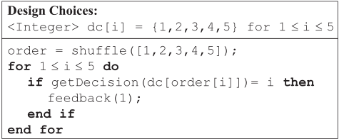
Figure 3 shows the code for benchmark 2. In this benchmark we are to make 5 design decisions between 1, 2, 3, 4 and 5, in a random order. If we choose alternative i the ith design choice (iteration), we receive a reward of 1. Here, the best decision depends on the number of design decisions made before, which is only known at runtime.

3 The focused variant, using the default parameter settings.

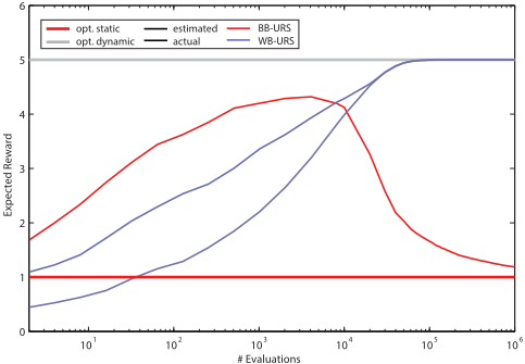
Figure 4 shows that WB-URS finds the optimal dynamic policy, which accumulates a reward of 5. This might surprise, since our optimizer is context oblivious. However, Sco does include minimal runtime information (partial configuration c0 2 C 0 ), which is sufficient to act optimally in this benchmark. BB-URS only considers static configurations, which are all as good, accumulating an expected reward of 1. Note that BB-URS also suffers from oc on this benchmark.

7 Related Research

This section lists prior-art on algorithm design, that can be viewed as following a white box approach. Rather than being complete, we attempt to characterize their nature and clarify how our work differs from theirs.

We consider designing algorithms in general (TMadp). Prior-art considers specific subclasses of algorithms (e.g. Divide & Conquer-algorithms [Lagoudakis and Littman, 2000], Evolutionary Algorithms [Eiben et al., 1999; Karafotias et al., 2014], Meta-heuristics [Burke et al., 2003], Constraint Satisfaction Programs [Epstein et al., 2002] etc). We reformulate this problem as an MDP. While some (e.g. [Lagoudakis and Littman, 2000; Karafotias et al., 2014]) informally suggest this could be done, they eventually formulate and solve a problem that is not Markovian. The Markovproperty is what enables us to generalize across runs, inputs and configurations in a theoretically sound manner. Also, note that the MDP formulation in [Lagoudakis and Littman, 2000] is far more black-box than ours (states represent independent sub-problems, actions correspond to algorithms).

Finally, there exists a vast body of research attempting to make/adapt design decisions at runtime. Well-known examples are reactive-search [Battiti et al., 2008] and selection hyper-heuristics [Burke et al., 2003]. Online adaptivity is indeed a key advantage of the white box approach, enabling better designs (see Section 4.2). However, to the best of our knowledge, prior-art does this outside of a proper theoretical framework, relying mostly on heuristics. Learning, if used at all, is done online, without generalization across runs and introduces a trade-off between exploration and exploitation. Benefits as such are often minimal and exploitation of learned knowledge requires very long/repetitive runs (e.g. an RL approach performs barely better than random in [Karafotias et al., 2014]). Furthermore, the RL problem these methods (often implicitly) solve, has a non-stationary environment, thus requiring us to learn faster than the environment changes. A proper theoretical framework is exactly what we propose in this paper. Note that in our formulation, online-learning is no prerequisite for online adaptivity, i.e. we can learn "what works when" offline and utilize this knowledge online.

8 Conclusion

In summary, this paper focuses on formulating the Algorithm Design Problem (ADP) in a general and formal manner (TMadp), describing/illustrating its potential benefits, without bias towards a particular solution approach, something prior-art, without exception, fails to do. The ADP as formulated in this work subsumes the algorithm selection, parametrization and dynamic adaptation problems, and as such might be foundational to enabling a more unified approach to automated algorithm design in the future. The MDPadp formulation is of particular interest, as it allows us to leverage the gamut of MDP solution approaches (e.g. RL) that have been proposed over the past six decades to do so.

While exploiting the full potential of the white box approach is a challenging endeavor and was beyond the scope of this paper, we believe that the envisioned benefits should make this a research track worth exploring. Furthermore, to convince the reader our approach is practical nonetheless, we have presented a concrete white box optimizer and used it to illustrate how white box information can be utilized to speed up the optimization process as well as improve the quality of the resulting design, on two illustrative microbenchmarks. Subject of future research is a white box optimizer, outperforming state-of-the-art algorithm configurators on real-world ADPs. Worst-case, if each configuration uniquely affects the execution on every input, we can do no better. Our objective is therefore to never do worse. Also subject of future research is a practical approach to profit from the (partial) observability of context during the design process. Finally, we wish to explore the potential of using this framework to analyze and compare heuristics (human-defined policies) commonly used to make design choices at runtime and how these can be used to inform the optimization process.

In the future, automated algorithm design will play an increasingly prominent role. Recently, multiple sources [Ansel et al., 2009; Hoos, 2012; Adriaensen et al., 2014] have independently advocated a PbO-like methodology to design algorithms. Simultaneously, many fields have in recent years suffered from an uncontrolled introduction of algorithmic variation. We expect that maturation of these fields will lead to a more controlled, modular, component-driven approach (e.g. Metaheuristic Optimization [Swan et al., 2015]). The question of which components to combine to solve a given problem will surely be one computers must help answering.

Acknowledgments

Currently, Steven Adriaensen is funded by a Ph.D grant of the Research Foundation Flanders (FWO).