Packing Graphs with ASP for Landscape Simulation

1 Introduction

An agricultural landscape describes the spatial organization of agricultural plots with their land-use (grass, wheat, corn, etc.). It can be characterized by the local arrangements (that we call co-locations) of crops in the landscape plots.

The development of computational tools for realistic landscape simulation remains a challenge. It requires to generate the plot boundaries as well as the land-uses. In this work, we are only interested in land-use generation, also known as the crop-allocation problem. Only few works have investigated the generation of realistic plots boundaries. For instance, [Le Ber et al., 2009] proposed to use tessellation to generate plots geometry.

Two types of approaches can be distinguished for land-use generation: simulation, based on decision processes and the so-called "neutral" process, based on learning. In [Akplogan et al., 2013], the authors use constraint programming to propose a plot map satisfying crop allocation constraints respecting the farmers' management choices. Such decision processes require precise knowledge in order to model the behavior of actors. This knowledge may be difficult to acquire. In contrast to this simulation-based approach, [Le Ber et al., 2009] propose a neutral process based on the reproduction of some learned landscape features, e.g. the spatial distribution of plot centroids. This kind of feature can easily be extracted from a real landscape by a spatial statistical process. The method introduced in [Lazrak et al., 2009] simulates land-use by learning crop co-location Hidden Markov Model (HMM) along a fractal curve and by generating new crop allocations from them. [Schaller et al., 2012] combines both approaches.

The present work investigates how to allocate the crops of a landscape by reproducing the representative co-locations, i.e. neighbor crops patterns, extracted from some real landscape. An agricultural landscape is represented by a plot graph where vertices represent plots and edges model the adjacency of two plots. Co-locations of the landscape are subgraphs of the plot graph. The simulation process has two main stages: 1) characterize a real landscape by extracting a set of representative co-locations and 2) build "realistic" land uses that combine representative co-locations.

Given a set of representative co-location patterns learned from some landscape in stage 1), the paper describes a method for completing stage 2), i.e. allocating crops in a new empty landscape by combining the given patterns. A constraint logic programming approach (more specifically Answer Set Programming - ASP) is proposed for its ability i) to solve combinatorial problems efficiently ii) to take into account expert knowledge for crop allocation.

2 A general framework for landscape simulation from co-locations

Our goal is to generate landscapes reproducing the landuse organization of some given real landscape. The general framework is illustrated in Figure 1. This paper focuses on steps in the dashed frame.

A landscape is formally represented by a graph G = hV↪E↪µ : V 7!Si where vertices of V represent plots, edges of E encode the adjacency of plots, S represents the crops (e.g. wheat, grassland, corn, etc.) and µ is an allocation function that assigns to each plot one crop from S.

We assume that frequent co-locations are representative of a landscape. In order to replicate some landscape spatial organization, the first step is, thus, the extraction of these colocations from a real landscape. Algorithm gSpan [Yan and Han, 2002] has been adapted to extract frequent co-locations in the form of attributed sub-graphs. The spatial organization of a co-location is extracted in a so-called structure that is represented as a non-attributed graph isomorphic to at least one co-location occurrence.

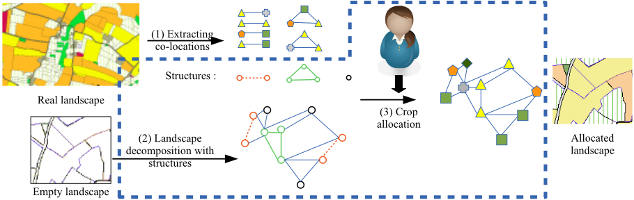
In a second step, the input bare landscape, i.e. a nonallocated plot graph, is divided into disjoint structure instances. The problem is to cover all vertices of the graph by non-overlapping instances.

Finally (third step), the process allocates crops to the plots of the new landscape, according to the crops in the co-location associated with the structure instances extracted from the original plot graph. In Figure 1, steps 2 and 3 are presented as sequential steps. Nonetheless, in our solving process they are solved simultaneously.

3 Graph packing with structures

This section introduces the specification of our specific problem of graph packing with generic structures. Graph packing with well-known graph families - e.g. the set of complete graphs of size n, ¶Kn♦ - has been studied in graph theory [Plummer and Lov´asz, 1986]. However, no algorithm has been proposed yet to solve efficiently the problem of graph packing with a set of structures having no specific topological properties.

Let G = hV↪Ei be an unlabeled and undirected graph. Without loss of generality, we consider only connected graphs, i.e. with at least one path between two vertices. Packing a non connected graph can be reduced to packing its connected components independently.

Let S be a set of connected graphs, called structures. Let ⇠ (resp. ⌧) denote the "isomorphic to" (resp. "not isomorphic to ") relation over graphs. We assume that 8S1↪S2 2 S ↪ S1 ⌧ S2.

An instance I of a structure S = hVS↪ ESi 2 S in a graph G is a sub-graph hVI ↪EI i of G such that VI ⇢V , EI ⇢ E and I ⇠ S. The set of instances is denoted I . The function s : I 7! S maps instances to structures. A graph packing of G with S is a set of instances IS ⇢ I such that each vertex of G is uniquely mapped to an instance vertex and conversely, each instance vertex is mapped to a single vertex in G. Moreover, if there exists an edge between two vertices in some instance then there is an edge between the mapped vertices in G:

• ÷ 8I 2 IS ↪ I = hVI↪EIi^VI ✓V ^EI ✓E^ s(I) 2 S
• ÷ 8I = hVI↪EIi 2 IS ↪8vI 2VI↪9!v 2V↪vI = v
• ÷ 8v 2V↪ 9!I 2 IS ↪ I = hVI↪EIi^9!vI 2VI↪vI = v

The size of a packing, denoted by ♣I ♣, is the number of instances in I . The graph-packing I of G is said to be optimal if its size is minimal.

Note that in the general case, the graph-packing issue may have no solution or multiple solutions. We assume hereafter that S contains the singleton graph. Consequently, for any graph, there is at least one trivial packing solution consisting of singletons.

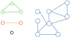
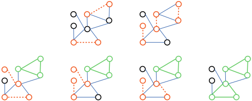
Example We consider the graph G and the set of structures S illustrated in Figure 2. S contains three structures: a pair (two connected vertices) displayed with a dashed edge, a triangle (three connected vertices) displayed with plain edges and the singleton graph. Figure 3 displays some correct packings of G.

4 Solving graph packing with ASP

ASP dates back from research on non monotonic logic and logic programming [Gelfond and Lifschitz, 1988]. An ASP program consists of Prolog-like rules l0 :- l1↪ ▷ ▷ ▷ ↪ lm↪not lm+1↪ ▷ ▷ ▷ ↪not ln, where each li is a literal. Such a rule states that l0 is proved to be true (l0 is in an answer set) if l1↪ ▷ ▷ ▷ ↪ lm are true and one can not prove that lm+1 ▷ ▷ ▷ ln are true. not stands for default negation. If the rule body is empty, l0 is a fact. A rule with an empty head specifies an integrity constraint. Together with model minimality, interpreting the program rules this way provides the stable model semantics, see [Gelfond and Lifschitz, 1990] for details. Grounding on this theoretical work, efficient implementations have been set up, cf. [Gebser et al., 2011]. An ASP system is the combination of a rich, yet simple, declarative modeling language with high-performance propositional solving capabilities relying on principles that led to fast SAT solvers. Given an ASP program, an ASP solver computes answer sets that are solutions of the encoded problem. To facilitate the use of ASP in practice, several extensions have been brought to the language along time, such as choice, cardinality, aggregates, weight expressions and optimization statements. In the sequel, we rely on the input language of the ASP system clingo [Gebser et al., 2015].

The main objective of this paper is to show the effectiveness and flexibility of ASP for the graph-packing problem stated in section 3. The reminder of this section provides a first encoding for solving the graph packing problem in ASP. The next section will present how to break symmetries in order to improve the program efficiency.

4.1 Problem representation

The input graph to be packed, G, is encoded with predicates vertex(X) stating that X is a vertex and edge(X,Y) stating that there exists an edge between vertices X and Y in graph G. The input structures S 2 S are encoded with atoms structure (S) (S is a structure of S), svertex(S,P) (P is a vertex of structure S) and sedge(S,P,Q) (there exists an edge between vertex P and vertex Q in structure S).

A graph packing solution consists of non overlapping structure instances that cover all the graph vertices. Instances are encoded by predicates instance and map describing the mapping of instance vertices to G vertices. instance(I,S) states that I is an instance of structure S and map(I, X, P) states that vertex P of instance I is mapped to vertex X in G.

4.2 A generate and test program

Listing 1 introduces an ASP program for the packing problem. It may be seen as a generate and test approach. The generation phase describes the space of all possible combinations of instances (lines 8-10) and, for each combination, it generates all possible mappings of instance vertices to graph vertices (lines 18-20). Line 1 ensures that graph edges are bidirectional since graphs are non-oriented.

1 edge(X,Y) :- edge(Y,X). 2 3 %additionnal graph features : graph size and stucture size 4 gsize (L) :- L = #count¶ N : vertex(N) ♦. 5 ssize (S, L) :- L=#count¶ N : svertex(S,N) ♦, structure(S) . 6 7 % INSTANCE GENERATION 8 1 ¶ instance (1,S) : structure(S) ♦ 1. 9 ¶ instance(I+1,S2) : S2>=S, structure(S2) ♦ 1 :- 10 instance(I ,S) , gsize (L), I<L. 11 12 % The total number of instance vertices must be 13 % equal to the number of vertices in the graph 14 :- NI=#sum¶ L,I : ssize (S,L), instance(I ,S) ♦, 15 gsize (NG), NG!=NI. 16 17 % MAPPING GENERATION 18 1 ¶ map(I, X, 0) : vertex(X) ♦ 1 :- instance(I , S) . 19 1 ¶ map(I, Y, Q) : edge(X, Y) ♦ 1 :- 20 instance(I , S) , sedge(S, P, Q), map(I, X, P). 21 22 % an instance vertex must be mapped to a single 23 % graph vertex 24 :- map(I, P, X), map(I, P, Y), X<Y. 25 % a graph vertex X must be mapped to a single 26 % instance vertex 27 :- map(I, X, ) , map(J, X, ) , I<J. 28 :- map( , X, P), map( , X, Q), Q<P. 29 % every graph vertex must be covered 30 :- not map( , X, ) , vertex(X). 31 32 %OPTIMIZATION 33 nbinstances(L) :- L=#count¶ I : instance(I , ) ♦. 34 #minimize¶ L : nbinstances(L) ♦.

Listing 1: Modeling graph-packing in ASP. See section 4.1 for predicate semantics.

Without a clever generation method, many equivalent instance sets are generated, differing only by the identifier assigned to the different instances. To avoid this, we impose that instances are ordered. Structure and instance identifiers are represented by integers. Lines 8-10 state that the identifiers of instances are ordered with respect to the order of the identifiers of their related structure. In addition, the constraint in lines 14-15 imposes that the total number of vertices from all the instances is equal to the number of vertices in the graph (given by predicate gsize (N)).

The mapping described by map atoms in lines 18-20 enforces an isomorphism between each instance and some subgraph of G: for each instance I containing a pair of map atoms, if there is an edge between the vertices in the structure associated with I then an edge should exist between the mapped vertices in G.

To avoid the generation of (some) equivalent mappings, differing only by the identifier of mapped vertices, a structure S = hVS↪ESi is modeled by a directed acyclic graph (DAG), such that for any vertex v 2VS, there exists an oriented path from a fixed root vertex v0 to v. The set of oriented edges defines a topological order for browsing efficiently the edges of this structure following a depth-first strategy.

Lines 18-20 implement such a depth-first search strategy in ASP. Line 18 states that the root vertex of instance I (vertex 0) is mapped to a unique graph vertex X. Lines 19-20 state that each vertex Q of some instance I, such that there is an edge from P to Q and such that P is mapped to graph vertex X, is mapped to a graph vertex Y such that there is an edge between X and Y. Atoms map generated this way define an isomorphism between VS and VI ⇢V, such that any edge of the structure instance is associated with an edge in G, linking the mapped vertices of VI .

Lines 24-30 constrain the mapping by not allowing missing or unmapped edges. If there is no edge between two vertices P and Q in some structure S, then there should not exist any edge between the corresponding vertices in the graph. We use inequalities X<Y (logically equivalent to X!=Y in these cases), because X<Y leads to smaller grounding. Some of these constraints could be redundant, e.g. lines 24 and 28 (only one is mandatory), but improve computation times. Finally, line 30 enforces that all the vertices of G are mapped.

The last part concerns optimization. Lines 33-34 keep only the optimal answer sets, i.e. the sets containing the minimum number of instances.

5 Breaking structure symmetries

Structure symmetries have a high impact on the combinatorial complexity of mapping since some structure can be mapped in several equivalent ways to a subgraph. Coping with such symmetries is a well known issue for ASP solvers [Drescher et al., 2011]. Symmetry breaking attempts to eliminate symmetric parts of the search space. In the case of structures, this corresponds to finding bijective transformations on their set of nodes (e.g. rotations) such that the structure is left invariant by this transformation. Such transformations are called automorphisms. This section presents an ASP modeling of the search for automorphisms and the way they are used in graph packing for symmetry breaking.

5.1 Graph automorphisms

A permutation of a set W is a bijection from W to itself. For example, [5↪2↪6↪1↪4↪3] is a permutation of [1↪2↪3↪4↪5↪6]. A permutation can be represented as a composition of disjoint exchange cycles: (1 ! 5 ! 4) (3 ! 6) = (1↪5↪4)(3↪6) for this example. Sym(W) is the set of all permutations of W.

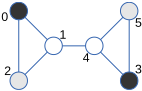
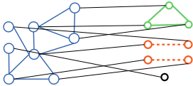
For an undirected graph G = hV↪Ei, a graph automorphism is a permutation of V that preserves adjacency. The set Aut(G) = ¶p 2 Sym(V) ♣ p(E) = E♦ equipped with the composition of permutations ◦ forms a group that describes all possible symmetries. Using composition, this group may be generated from a few elements. For instance the group of symmetries for the graph in Figure 5 may be generated by 3 automorphisms: (0↪2), (3↪5), and (0↪3)(1↪4)(2↪5). A structure has some symmetries if there is at least one non-identity permutation in the automorphism group.

Now, we relate automorphisms to the packing issue. Let G be a graph to be packed and S a structure. Let GS denote a subgraph of G induced by an isomorphism f between S and GS. Let p be an automorphism of S, then p◦f is also an isomorphism between S and GS. In such a case, Listing 1 would generate several answer sets corresponding to these automorphisms for the same solution.

5.2 Finding automorphism symmetries in ASP

Our ASP encoding for finding automorphism symmetries is based on equitable partitions, as in the nauty program [McKay and Piperno, 2014]. An equitable partition consists of clusters of vertices, such that all vertices of a cluster have exactly the same number of neighbours in each cluster. An example of equitable partition is provided in Figure 5. Each cluster is displayed with a different color: each black vertex has 1 neighbor among grey vertices and 1 among white vertices and a similar observation can be done for white and grey vertices. Equitable partitions enable to reduce the search for automorphisms since it is a necessary condition for the cycles of the corresponding permutation. However, it is not sufficient and the graph isomorphism has to be verified (simple statement not shown in Listing 2).

Listing 2 proposes an ASP encoding to search the space of equitable partitions and permutations (symsedge is the symmetric version of sedge). This encoding is an elegant alternative for the main task of nauty.

5.3 Breaking structure symmetries in ASP

Consider now a structure S with vertices VS and a graph G. The mapping between S and G is represented by an isomorphism f. To each permutation p 2 Aut(S) found by the previous program may be associated some validity constraints to be satisfied by f. Permutations are ordered partitions: the idea is to consider consecutive pairs of vertices in a cycle and to impose a compatible ordering in f. This will reduce the number of admissible f. More formally, an isomorphism f will be "valid for a pair (u↪v) in a permutation p 2 Aut(S)" iff p has a cycle with two consecutive elements u and v and f verifies u < v ) f(u) < f(v).

Let p be a permutation that interchanges two elements, u and v and leaves the remaining elements unchanged. Then f◦

1 %Partition: vertex N of structure S belongs to cluster B 2 1 ¶ clust (S,B,N): svertex(S,B) ♦ 1 :- svertex(S,N). 3 cluster (S,B) :- clust (S,B,N). 4 5 %The number of neighbours of vertex N in cluster B is K 6 nbneighb(S,N,B,K) :- svertex(S,N), cluster (S,B), 7 K=#count¶M: symsedge(S, M, N), clust(S,B,M) ♦. 8 9 %K is a type of cluster B1 with respect to cluster B2 if an element of B1 has K neighbours in B2 10 type(S,B1,B2,K) :- clust (S,B1,M), nbneighb(S,M,B2,K). 11 12 %Equitable partition : each cluster pair has a unique type 13 :- 2 ¶ type(S,B,X,L) ♦, cluster (S,B), cluster (S,X). 14 15 %Permutation=Ordered partition: N2=succ(N1) in cluster B 16 1 ¶ map(S,B,N1,N2): block(S,B,N2) ♦ 1 :- block(S,B,N1).

Listing 2: Symmetry search through equitable partitions.

p and f are two isomorphisms such that 8w 2VS↪w 6= u↪w 6= v↪ f◦p(w)=f(w), f◦p(v)=f(u) and f◦p(u)=f(v). Then, if u < v one and only one isomorphism will be valid for p.

The program looks for automorphisms that maximize the number of such constraining pairs. More generally, cycles larger than 2 may be constrained by more than one pair. However, adding a validity constraint for each of the possible pairs may be unsatisfiable. The program looks for an automorphism that maximizes the number of constraining pairs while leading to a valid isomorphism, i.e. an isomorphism valid for all constraining pairs.

In our example, (0↪2) and (3↪5) are two permutations for which f is valid that will give two vertex constraints. In our ASP encoding of graph packing, validity constraints are encoded by atoms ordpair(S,P,Q) meaning that vertices P and Q must be ordered in structure S. The following rule enforces the constraint in the program:

:- instance(I ,S) , ordpair(S,P,Q), map(I, X, P), map(I, Y, Q), Y<=X.

ordpair/3 atoms are automatically generated from permutations. In our example, they are generated for pairs (0↪2), (3↪5), and also (1↪4), derived from (0↪2), (3↪5), and (0↪ 3)(1↪ 4)(2↪ 5).

6 Generating crop allocation

The graph-packing process decomposes the graph into small structures. The crop allocation process uses these structures to allocate crops to all vertices in the graph. An "allocated structure" is a structure instance where each vertex has been assigned a land use. Note that there may exist several allocated structures related to the same (bare) structure.

6.1 Crop allocation

The following predicates are introduced to implement crop allocation: attstruct (AS,S): AS is an allocated structure isomorphic to structure S; attvertex (AS,P,A): vertex P of structure AS is allocated with crop A; gvertexf(N,A): crop A is allocated to vertex N, at initialization; gvertex(N,A): crop A

1 %fixed crops 2 gvertex(N,A) :- gvertexf(N,A). 3 allocated (N) :- gvertexf(N,A). 4 5 %free plots to allocate 6 1 ¶ selectedAS(AS,I): attstruct (AS,S) ♦ 1 :- 7 instance ( I , S) . 8 9 gvertex(N,A) :- attvertex (AS,P,A), selectedAS(AS,I), 10 map(I,N,P), not allocated (N). 11 :- gvertex(N,A), allocated (N), attvertex (AS,P,B), 12 map(I,N,P), selectedAS(AS,I), instance(I ,S) , A!=B.

Listing 3: Crop allocation.

is allocated to graph vertex N, by crop allocation; selectedAS( AS,I): allocated structure AS is associated with instance I.

Crop allocation consists in generating atoms of the gvertex /2 predicate. The land use of some plots, such as roads, buildings, woods, can be static and should not be re-computed. Lines 2-3 of Listing 3 generate gvertex/2 atoms in such cases. Lines 9-10 generate gvertex/2 atoms in the other case. For each graph vertex, the crop is allocated with the crop associated with the corresponding vertex in the allocated structure. Lines 11-12 enforce consistency of initially allocated crops and mapped allocated structures: a crop allocated to some vertex must be identical to the crop initially allocated to this vertex, if any.

6.2 Modeling expert constraints

Beyond allocated structures modeling crop co-locations, experts can add local or global constraints. Listing 4 illustrates the versatility of such constraints. Local constraints coerce or forbid the presence of some crops in the neighborhood of some plot. For instance, farmers used to not grow cereals close to forests to avoid damages by wild animals, such as boars or roes. This constraint is formulated in Line 2 of Listing 4. Global constraints concern aggregates related to the whole crop allocation. Line 14 illustrates a global constraint on the overall surface allocated with wheat. The predicate surf /2 giving the surface of each plot has been added.

1 %No corn plot (8) neither wheat plot (7) close to forest (3) 2 :- edge(X,Y), gvertex(X,8), gvertex(Y,3). 3 :- edge(X,Y), gvertex(X,7), gvertex(Y,3). 4 %Not less than 5 wheat plots 5 ngvertex(L,OS) :- L=#count¶ X: gvertex(X,OS) ♦. 6 :- ngvertex(L,7) , L<5. 7 %No additional plot with buildings (11) 8 :- gvertex(X,11), not allocated (X). 9 %A corn plot covers at least 5000 m2 10 :- gvertex(X,8), not allocated (X), surf(X,S), S<5000. 11 % lusurf (C,A): A is the total area of plots with land use C 12 lusurf (C,A) :- vertex(X), landuse(C), 13 A=#sum¶ S: gvertex(X,C),surf(X,S) ♦. 14 %At least 100000m2 is allocated with wheat 15 :- lusurf (7,S) , S<100000.

Listing 4: Example of expert rules.

7 Experiments

The ASP solver clingo (version 4.5) [Gebser et al., 2011] was used on a desktop computer without parallelism for a quantitative evaluation of the efficiency of packing programs. 7*40 graphs 1 of size going from 16 to 61 vertices were randomly generated with a fixed edge density set to 1.2.

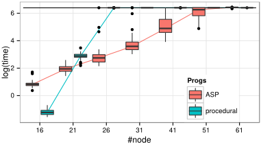
Figure 6 presents the computation times for packing random graphs with 10 structures containing at most 4 edges (5 vertices). The packing was solved with two methods: the "ASP" program (see Listing 1) without symmetry breaking and a "procedural" program that implements a complete search with backtracking. The horizontal dotted line represents the timeout of 10 min.

Figure 6 shows that computation time of the procedural approach is comparable with our approach for small graphs (sizes 16 and 21), but increases very quickly with the graph size. Beyond size 26, the procedural approach cannot solve the packing within the timeout period whereas our ASP encoding does. For graphs of size larger than 31, ASP runs several orders of magnitude faster than the procedural program.

The efficiency of symmetry breaking was studied on packing with a set of two structures: the singleton and the line of three vertices (S2). Figure 7 plots the normalized difference of computation times with and without symmetry breaking. If this difference is above 0, taking symmetries into account is slower than ignoring them. This can be observed for small graphs. However, we can notice that the larger the graphs, the closer to 0 the mean is: symmetries do not significantly increase the computation time for large graphs. The negative skewness of the distribution of time differences shows that symmetry breaking is more efficient on larger graphs. It is worth noting that 12 problem instances 2 among the 200 instances could only be solved using symmetries.

The graph packing encoding has been integrated in a crop allocation tool. In this software, the expert provides a plot geometry in a standard geographical format (standard shapefiles), a set of allocated structures and his own expert rules. These files are transformed into ASP facts. Then, the solver proposes crop allocations and, finally, an allocated landscape is generated in a geographical format. Experiments have been done for 4 real landscapes containing up to 200 plots with edge densities of about 3. The software received a positive feedback from experts.

1 all programs and instances can be found at https://sites.google.com/site/graphpacking/.

2 0 instances of size 21, 3 of size 31, 1 of size 41, 2 of size 51 and 6 of size 61.

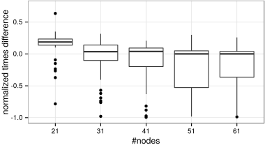
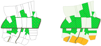
Figure 8 illustrates a practical application of crop allocation on a landscape containing 45 plots. Roads, forests and buildings were allocated initially. The crop-allocated landscape satisfies both the crop co-locations defined in allocated structures and expert rules. This landscape is one solution among all possible solutions. We can notice that wheat have been allocated only to the large plots that are not close to forests, as specified by expert rules.

8 Conclusion

In this article, we have presented the problem of crop allocation with respect to co-locations. We have formalized the problem as a graph-packing problem which is known to be highly combinatorial. An ASP program has been proposed to solve the graph-packing problem and its performance has been assessed. Symmetry breaking was introduced to improve the efficiency of the basic solution. Solving the most difficult instances was significantly faster with symmetry breaking. This is highly valuable to a user who has to cope with large graphs and complex constraints. From a qualitative point of view, the resulting allocated landscapes are quite realistic. The realism can be easily enforced by adding expert rules stating local or global constraints. ASP is quite adapted for adding such background knowledge.