Counting Linear Extensions of Sparse Posets

1 Introduction

Determining the number of linear extensions of a given poset (equivalently, topological sorts of a directed acyclic graph) is a fundamental problem in order theory, with applications in areas such as sorting [Peczarski, 2004], sequence analysis [Mannila and Meek, 2000], convex rank tests [Morton et al., 2009], preference reasoning [Lukasiewicz et al., 2014], and learning probabilistic models from data [Wallace et al., 1996; Niinim¨aki and Koivisto, 2013].

Brightwell andWinkler [1991] showed that exact counting of linear extensions is #P-complete and therefore not tractable for general posets unless P = NP. By dynamic programming over the lattice of upsets (see, e.g., De Loof et al. [2006]) linear extensions can be counted in time O(♣U♣ · w), where U is the set of upsets and w is the poset width. This implies the worst case bound O(2nn) for a poset on n elements, which to our knowledge is the best to date. Though exponential in n, the algorithm can be very fast for posets with few upsets. In particular, it holds that ♣U♣ = O(nw ), since every poset can be partitioned into w chains and an upset can be specified by the number of elements it contains from each chain. Hence the algorithm runs in polynomial time for bounded width. Conversely, the set U can be very large when the order relation is sparse, which raises the question if sparsity can be exploited for counting linear extensions faster.

⇤This work was supported in part by the Academy of Finland, grants 125637, 255675, and 276864.

In this work we present two approaches to counting linear extensions that target sparse posets in particular. In Section 2 we augment the dynamic programming algorithm by splitting each upset into connected components and then computing the number of linear extensions by recursing on each component independently. We also survey previously proposed recursive techniques for comparison.

In Section 3 we show that the problem is solvable in time O(nt+4 ), where t is the treewidth of the cover graph. While our result stems from a well-known method of nonserial dynamic programming [Bertel`e and Brioschi, 1972], known as variable elimination and by other names [Dechter, 1999; Koller and Friedman, 2009, Chap. 9] global constraints in the problem hamper its direct, efficient use. To circumvent this obstacle, we apply the inclusion-exclusion principle to translate the problem into multiple problems without such constraints, which are then solved by variable elimination.

In Section 4 experimental results are presented to compare the two algorithms against previously known techniques. We conclude with some open questions in Section 5.

1.1 RelatedWork

A number of approaches for breaking the counting task into subproblems have been considered before. Peczarski [2004] reports a significant gain on some families of posets by recursively decomposing them into connected components and so called admissible partitions; however, this procedure has an unknown asymptotic complexity. Li et al. [2005] present another algorithm that recursively splits a poset into connected components and so called static sets.

Besides bounded width, polynomial-time algorithms exist for several restricted families of posets such as series-parallel posets [M¨ohring, 1989], posets whose cover graph is a polytree [Atkinson, 1990], posets with a bounded decomposition diameter [Habib and M¨ohring, 1987], and N-free posets of a bounded activity [Felsner and Manneville, 2014].

Fully polynomial time randomized approximation schemes are known for estimating the number of linear extensions [Dyer et al., 1991; Bubley and Dyer, 1999].

For listing all linear extensions there exist algorithms that spend O(1) time per linear extension on average [Pruesse and Ruskey, 1994] and in the worst case [Ono and Nakano, 2007].

1.2 Preliminaries

A partially ordered set or a poset is a pair (P↪P ), where P is a set and P is an order relation on P, that is, a binary relation that is reflexive, antisymmetric, and transitive. The elements (a↪ b) of P are denoted simply a P b. Elements a↪ b 2 P are comparable if a P b or b P a, and otherwise incomparable, denoted a♣♣P b. We say that a is a predecessor of b, denoted a <P b, if a P b and a 6= b. Dually, b is called a successor of a. An element with no predecessors or successors is a minimal or maximal element, respectively.

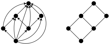
We say that b covers a, denoted a ≺P b, if a <P b and there is no c 2 P such that a <P c <P b. A poset is uniquely identified by the cover relation ≺P and can be presented by the cover graph (Figure 1), usually drawn as a Hasse diagram, where an edge upwards from a to b implies a ≺P b.

A linear extension of an n-element poset P is a bijection σ : P ! [n] that respects the order P , that is, a P b implies σ(a)  σ(b) for all a↪ b 2 P . Here and henceforth the bracket notation [n] denotes the set ¶1↪ ▷ ▷ ▷ ↪ n♦. An equivalent condition is that σ respects the cover relation, i.e., a ≺P b implies σ(a) < σ(b). The number of linear extensions of P will be denoted `(P).

A set of elements A ✓ P is called a chain if all pairs of elements in A are comparable and an antichain if no pairs are comparable. The width of P, denoted w(P) or simply w, is the size of the largest antichain. A downset is a set of elements D ✓ P such that for all b 2 D↪ a 2 P it holds that a <P b implies a 2 D. Dually, an upset is a set U ✓ P such that for all a 2 U↪ b 2 P it holds that a <P b implies b 2 U.

We will typically identify a poset simply with the set of elements P. Further, any subset A ✓ P will be implicitly treated as a subposet (A↪A) of P, that is, for all a↪ b 2 A it holds that a A b if and only if a P b.

2 Counting by Recursion

We begin with a brief survey of known methods for counting linear extensions by recursively decomposing the task into subproblems. For the remainder of the section consider an arbitrary non-empty poset P .

First, observe that each linear extension of P begins with some minimal element x 2 P , and the number of extensions that begin with x equals `(P ∩ x). Therefore, we have that

where min(P) denotes the set of minimal elements of P .

A direct evaluation of recurrence 1 corresponds to enumeration of all linear extensions. It is easy to see that the sets U ✓ P for which `(U) is computed are exactly the upsets of P. If we store these intermediate results so that each is computed only once, we obtain the O(♣U♣ · w) time dynamic programming algorithm. The number of minimal elements is bounded by w and they are found in O(w) time by simple bookkeeping.

By symmetry recurrence 1 still holds if x are taken over the maximal elements instead, in which case the algorithm will run over the downsets of P. Since downsets are exactly the complements of upsets, the running time is unchanged.

Second, we consider the admissible partitions used by Peczarski [2004], formalized slightly differently here. For an arbitrary element x 2 P, we say that a partition of P ∩ x into a pair of sets (D↪ U) is admissible if D is a downset that contains all predecessors of x (and U an upset that contains all successors of x). Equivalently, a partition is admissible if and only if there is at least one linear extension σ such that σ(d) < σ(x) < σ(u) for all d 2 D and u 2 U. Choosing a linear extension of P is equivalent to choosing such a partition and ordering D and U independently. Thus, we have that

where (D↪ U) runs over all admissible partitions.

While this holds for any choice of x 2 P, not all choices are equally efficient. In general, it is preferable to choose an x such that the number of admissible partitions is minimized, which is exactly when P ∩ x has the maximum number of elements comparable with x.

Third, we consider the decomposition into static sets. We say that a non-empty set of elements S ⇢ P is a static set if every element in S is comparable with every element in P ∩ S and if no proper subset of S has this property. It is known [Li et al., 2005] that either P has no static sets, or there exists a unique partition of P into static sets S1↪ ▷ ▷ ▷ ↪ Sk. If the partition exists, a linear extension is obtained by ordering each Si independently, and therefore it holds that

Li et al. give an efficient algorithm that either finds the partition or determines that it does not exist.

Finally, if the graph representation of P is disconnected, i.e., if P can be partitioned into sets A and B such that a♣♣P b for all a 2 A and b 2 B, then taking a linear of extension of P is equivalent to ordering A and B independently and then interleaving them. Thus, in this case we have

Each of the rules 1-4 breaks the poset into one or more subposets whose linear extensions are counted recursively. It is easy to see that some rules are more effective for breaking certain kinds of subposets into parts than others, which suggests an algorithm that uses a combination of multiple rules.

One such algorithm was given by Peczarski [2004] who applies rule 4 whenever the poset is disconnected and rule 2 otherwise. Li et al. [2005] propose another algorithm, which applies rules 4 and 3 (in this order) when possible and falls back to enumeration when neither rule is applicable.

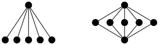
We propose an algorithm that augments the dynamic programming over upsets by applying rule 4 whenever the poset is disconnected and rule 1 in all other cases. When combining these two rules, we observe that it can make an exponential difference whether rule 1 is applied to minimal or maximal elements. For instance, consider a poset on n elements with n - 1 minimal elements (Figure 2, left) and notice that all of its upsets are connected. Therefore, if rule 1 is applied to minimal elements, rule 4 will never be applicable and the algorithm needs to consider O(2n ) upsets separately. On the other hand, if we remove the lone maximal element, the remainder of the poset breaks into singletons, and linear extensions are efficiently counted by applying rule 4.

Given an arbitrary poset P, it is not obvious which choice of rule 1 leads to a smaller number of subproblems that need to be solved. A very simple heuristic is to remove minimal elements if P has less minimal than maximal elements, and vice versa. We also propose a second heuristic that computes an estimate e(P) of the number of subproblems and makes the choice for which the estimate is smaller. The estimate is computed recursively as follows. If P is connected, we set e(P) = 2♣M♣ +e(P ∩M), where M is the set of minimal (respectively, maximal) elements of P. If P has the connected components P1↪ ▷ ▷ ▷ ↪ Pk, we set e(P) = e(P1)+· · ·+e(Pk). The intuition here is that for a connected poset we must (roughly) consider all subsets of minimal elements and then solve the subproblems in the remaining poset.

In certain cases (e.g. Figure 2, right) it can be effective to alternate the choice between minimal and maximal elements. However, our preliminary experiments suggest that on most posets it is preferable to make the choice once only and then apply it consistently. Intuitively this is because changing the choice breaks the property that all subproblems are either upsets or downsets, thus expanding the total space of possible subproblems. In practice this means that the recursion cannot reuse already computed subproblems as often, thus requiring a greater number of subproblems to be solved.

We also consider augmenting the algorithm further by applying rule 3 when possible. This can also be seen as an improvement of the algorithm of Li et al. where the raw enumeration is replaced by rule 1.

In Section 4 we present an experimental comparison of these proposals against other recursive algorithms. We will show in particular that on randomly generated posets both of the suggested heuristics almost always pick the better choice.

3 Counting by Variable Elimination

In this section we show the following result.

Theorem 1 Given a poset P, the number `(P) can be computed in time O(nt+4 ), where n = ♣P♣ and t is the treewidth of the cover graph of P.

We give a proof in the form of an algorithm. The key idea is to formulate the counting problem as a sum of products that factorize over the edges in the cover graph, and then apply the variable elimination scheme (see, e.g., Dechter [1999]) for computing the sum.

Let (P↪P ) be a poset on n elements. To simplify notation, we assume without loss of generality that P = [n]. On all (not necessarily bijective) mappings of form σ : [n] ! [n], define the function

where we define '(x↪ y) = 1 if x < y and '(x↪ y) = 0 otherwise. Recall that a linear extension of P is a bijection σ : [n] ! [n] that respects the cover relation ≺P . Therefore, for all bijections σ : [n] ! [n] it holds that Φ(σ) = 1 if σ is a linear extension and Φ(σ) = 0 otherwise. As a consequence, we have that

This form does not immediately admit variable elimination due to the global constraint that σ must be bijective. By applying the inclusion-exclusion principle, we can rewrite the sum as

which removes the undesired constraint from the inner sum but introduces a summation over all subsets of [n]. We now make use of the property of Φ that for all X ✓ [n] of fixed size k = ♣X♣ there are equally many ⌧ : [n] ! X such that Φ(⌧) = 1. Hence, it suffices to sum over all possible k:

The inner sum is now of the desired form

where we have expressed the summation over ⌧ : [n] ! [k] as a sum over the variables ⌧1↪ ▷ ▷ ▷ ↪ ⌧n, each of which runs over the values 1↪ ▷ ▷ ▷ ↪ k. A summation problem of this form is associated with an interaction graph, an undirected graph on the variables ⌧1↪ ▷ ▷ ▷ ↪ ⌧n, where two variables are joined by an edge if there is at least one function '(⌧i↪ ⌧j) in the product that depends on both of them. It is well known that with variable elimination such a sum can be computed in time polynomial in n and exponential in the treewidth t of the interaction graph, which in this case is exactly (the undirected variant of) the cover graph of P .

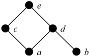
To establish the exact running time of our algorithm, we illustrate variable elimination with a simple example. Consider a poset on the elements ¶a↪ b↪ c↪ d↪ e♦ with a cover graph as shown in Figure 3. In this example the summation task is

where we have picked the elimination ordering d↪ e↪ a↪ b↪ c for the variables. Variables are summed out in the reverse order from right to left. To eliminate c, we organize the sum as

placing every function that does not depend on c outside the inner sum. The set of functions that do depend on c is called the bucket of c. Carrying out the inner summation produces a new function λc(a↪ e) = Pc '(a↪ c) '(c↪ e) that depends on every variable appearing in the bucket except c.

We put the new function in place of the sum and continue eliminating variables in this manner,

until we are left with a constant function whose value equals expression 5.

We first analyze the time required to eliminate a single variable x. Let m be the number of functions in the bucket of x and let q be the number of variables at least one of the functions depends on. From a computational point of view every function is simply an array that contains a value for each instantiation of its domain. Hence, eliminating x to produce λx involves iterating over all kq instantiations of the q variables, and for each instantiation the product of all m functions is computed. Thus eliminating x requires O(kq · m) time.

It is immediate that m = O(n), since in the beginning at most n - 1 functions depend on x and variable elimination produces at most n - 1 other such functions. On the other hand, the maximum value of q over all variables depends on the elimination ordering and is called its induced width. An elimination ordering is called optimal if it has the minimum induced width among all possible orderings. It is known that the induced width of an optimal elimination ordering is exactly t + 1 [Dechter, 1999]. Thus, given such an ordering, eliminating all n variables takes O(n2 · kt+1 ) time. Due to the inclusion-exclusion, expression 5 is evaluated by variable elimination for all k = 1↪ ▷ ▷ ▷ ↪ n, which brings the final running time to O(nt+4 ).

It remains to note that an optimal elimination ordering can be found in O(nt+2 ) time [Arnborg et al., 1987].

4 Experiments

We have implemented all algorithmic techniques described in Sections 2 and 3 for experimental evaluation. The following five (combinations of) techniques were considered:

• ÷ R1: Dynamic programming over upsets (rule 1 only).
• ÷ R24: The algorithm of Peczarski (rules 2 and 4).
• ÷ R14: Our proposal (applies rules 1 and 4).
• ÷ R134: Applies rules 1, 3, and 4.

For R14 we consider the following two variants:

• ÷ VEIE: Variable elimination via inclusion-exclusion.
• ÷ R14-a: The simple heuristic is used to decide whether rule 1 is applied to minimal or maximal elements.
• ÷ R14-b: The recursive heuristic is used instead.

For comparison, we also consider R14-best and R14-worst, two hypothetical variants of R14 that always make the best or the worst choice, respectively.

All posets used in these experiments were produced by randomly sampling directed acyclic graphs (DAGs) and taking for each DAG the corresponding partial order. The program LEcount, 1 comprising all implementations, was written in C++ and run on machines with Intel Xeon E5540 CPUs. Hashing was used in all implementations for storing the computed subproblems. All algorithms were given up to 20 minutes of CPU time and 30 GB of RAM on each poset.

4.1 Recursive Algorithms

In the first set of experiments we compare the first four algorithms against each other.

We generated two classes of sparse DAGs, parameterized by the number of vertices n 2 ¶30↪ 32↪ 34↪ ▷ ▷ ▷ ↪ 100♦ and a density parameter k 2 ¶2↪ 3↪ 4↪ 5↪ 6♦. In both classes a DAG was generated by picking a random ordering on the vertices and then adding edges compatible with the ordering. In the first class k is the expected average degree, achieved by adding each possible edge with probability k◁(n - 1). In the second class k is the maximum indegree, achieved by choosing for each vertex at most k parents among the preceding vertices in the ordering. This class is motivated by applications in learning Bayesian networks [Niinim¨aki and Koivisto, 2013], where the indegree is typically bounded.

We also generated a third class of dense bipartite graphs on n 2 ¶30↪ 32↪ 34↪ ▷ ▷ ▷ ↪ 60♦ vertices and a density parameter p 2 ¶0▷2↪ 0▷5♦. These were produced by splitting the vertices into two sets A and B of size n◁2 and adding the edge (a↪ b) for all a 2 A and b 2 B with probability p.

1 The LEcount program and all experiment posets are available at www.cs.helsinki.fi/u/jwkangas/lecount/.

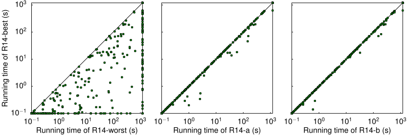
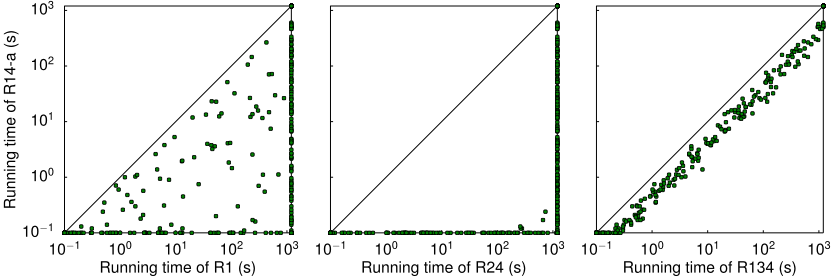
A comparison between the variants of R14 is presented in Figure 4. As suggested earlier, the choice between removing minimal or maximal elements has a huge impact on performance. It turns out, however, that even the simple heuristic is able to pick the better choice for a vast majority of random posets. The recursive heuristic improves upon this even further and appears to deviate less from the better choice even when it makes a mistake.

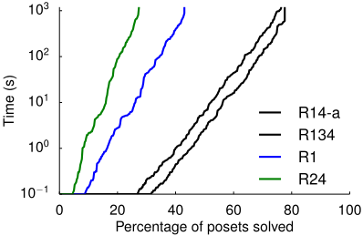
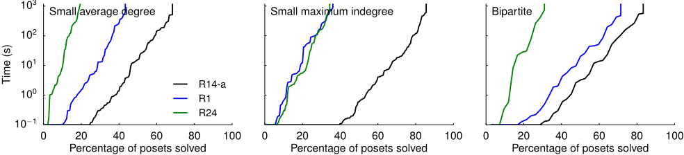
In light of this we only compare the variant R14-a to the other recursive algorithms (Figures 5 and 6). We observe that R14-a outperforms the other algorithms on every poset of the three classes. It beats R24 by a large margin and greatly improves upon the baseline set by R1, suggesting that rule 1 is in general better equipped for breaking a poset into connected components than rule 2. In algorithm R134 we used the simple heuristic for rule 1 to make it directly comparable with R14-a. A closer analysis of this algorithm reveals that rule 3 was applicable only to a handful of subproblems and thus could not compensate for the overhead of detecting static sets. We conclude that the addition of rule 3 does not improve upon the performance on R14.

The advantage of R14 over the other algorithms is most pronounced on the posets of bounded indegree (Figure 7). For the dense bipartite graphs its behavior is closer to R1 as most of the subposets are connected.

4.2 Variable Elimination

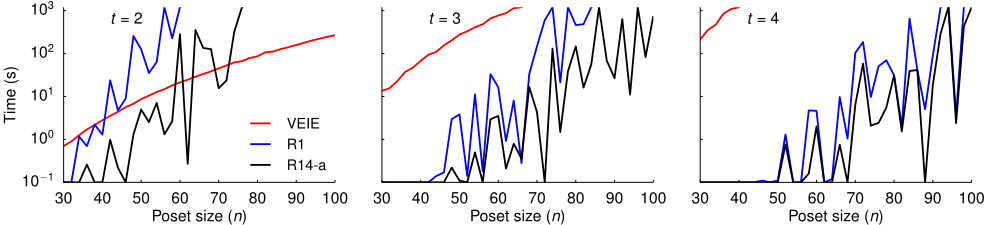
In the second set of experiments we compare the variable elimination algorithm VEIE against R14 and R1 on a set of grid trees on n 2 ¶30↪ 32↪ 34↪ ▷ ▷ ▷ ↪ 100♦ vertices and treewidth t 2 ¶2↪ 3↪ 4♦. Such a grid tree is constructed by randomly joining t by t grid posets along the edges, orienting the edges so that no directed cycles are introduced. Finding an optimal elimination ordering for a grid tree is easy and this step is omitted from the evaluation.

For a fixed value of t the running time of VEIE exhibits the expected polynomial behavior with respect to n (Figure 8). By contrast, the recursive algorithms are highly sensitive to other features of the poset structure and therefore display more erratic running times. On average their behavior is still exponential, allowing VEIE to surpass them on sufficiently large posets of low treewidth. We can observe this happening for t = 2, but for larger treewidth even R1 remains faster within the 20-minute time limit. We remark that the recursive algorithms typically run out of memory around this point, thus making VEIE the most viable option thereafter.

5 Conclusion

We have proposed two algorithms for counting linear extensions of posets, exploiting recursive decomposition into connected components and low treewidth, respectively. We demonstrated with experiments that the recursive algorithm beats previously proposed methods on a range of both sparse and dense posets, and that for large posets of low treewidth our second algorithm can be even faster. We also showed that simple heuristics often suffice to determine the better variant of the recursive algorithm.

As a conclusion, we raise some questions for future work. First, we note that one can easily construct specific examples where our recursive algorithm performs poorly compared to the other techniques. For instance, the poset in Figure 2, right, and larger posets with a similar structure, can be effectively decomposed into admissible partitions or static sets, whereas our algorithm requires an exponential time. While this is a very extreme example, it is natural to ask if there are notable classes of posets where the counting problem is nontrivial but solved effectively by applying multiple recursive techniques together. In particular, does any such class benefit from using both variants of rule 1 together, an approach that we rejected in general? Can further generalizations of rule 1 (e.g. Edelman et al. [1989]) yield even faster algorithms?

Second, the derivation of our O(nt+4 ) time algorithm required the trick of running variable elimination through inclusion-exclusion to avoid global constraints. Is this the natural best way to deal with the constraints or can a direct dynamic programming over a tree decomposition yield an equally or more efficient algorithm?

Lastly, in terms of parameterized complexity [Downey and Fellows, 2012], the running time of form nf(t) places the problem of counting linear extensions in the class XP when parameterized by the treewidth of the cover graph. A strictly better running time of form f(t) ·nO(1) would place the problem in the class FPT or fixed-parameter tractable. Does such an algorithm exist for the treewidth of the cover graph or some other poset parameter?

Acknowledgments

We would like to thank the anonymous reviewers for expanding our knowledge on related literature and other valuable comments for improving the presentation.