
Improved Heuristic and Tie-Breaking for Optimally Solving Sokoban
Proceedings of the Twenty-Fifth International Joint Conference on Artificial Intelligence. Pages 662-667.
Abstract
We present a novel admissible pattern database heuristic (D) and tie-breaking rule (L) for Sokoban, allowing us to increase the number of optimally solved standard Sokoban instances from 20 to 28 and the number of proved optimal solutions from 25 to 32 compared to previous methods. The previously best heuristic for Sokoban (I) used the idea of an intermediate goal state to enable the effective use of pattern database heuristics in transportation domains, where the mapping of movable objects to goal locations is not fixed beforehand. We extend this idea to allow the use of multiple intermediate goal states and show that heuristic I is no longer effective. We solve this problem and show that our heuristic D is effective in this situation. Sokoban is a well-known single-agent search domain characterized by a large branching factor, long solution lengths, and the presence of unsolvable states. Given the exponential growth in the complexity of standard Sokoban instances, the increase in the number of optimally solved instances represents a major advance in our understanding of how to search in extremely large search spaces.
- [Culberson and Schaeffer, 1996] Joseph C. Culberson and Jonathan Schaeffer. Searching with pattern databases. In Cana- dian Conference on Artificial Intelligence, pages 402-416, 1996.
- [Culberson, 1999] Joseph C. Culberson. Sokoban is PSPACE- Complete. In Fun With Algorithms, pages 65-76, 1999.
- [Edelkamp, 2001] Stefan Edelkamp. Planning with pattern databases. In European Conference on Planning, pages 13-24, 2001.
- [Felner et al., 2004] Ariel Felner, Richard E. Korf, and Sarit Hanan. Additive pattern database heuristics. J. Artificial In- telligence Res., 22:279-318, 2004.
- [Felner et al., 2007] Ariel Felner, Richard E. Korf, Ram Meshu- lam, and Robert C. Holte. Compressed pattern databases. J. Artificial Intelligence Res., 30:213-247, 2007.
- [Hart et al., 1968] Peter E. Hart, Nils J. Nilsson, and Bertram Raphael. A formal basis for the heuristic determination of mini- mum cost paths. IEEE Trans. Systems Science and Cybernetics, 4(2):100-107, 1968.
- [Holte et al., 2006] Robert C. Holte, Ariel Felner, Jack Newton, Ram Meshulam, and David Furcy. Maximizing over multiple pattern databases speeds up heuristic search. Artificial Intelli- gence, 170(16-17):1123-1136, 2006.
- [Hüffner et al., 2001] Falk Hüffner, Stefan Edelkamp, Henning Fernau, and Rolf Niedermeier. Finding optimal solutions to Atomix. In KI: Advances in Artificial Intelligence, pages 229- 243, 2001.
- [Junghanns and Schaeffer, 2001] Andreas Junghanns and Jonathan Schaeffer. Sokoban: Enhancing general single- agent search methods using domain knowledge. Artificial Intelligence, 129(1-2):219-251, 2001.
- [Korf and Felner, 2002] Richard E. Korf and Ariel Felner. Dis- joint pattern database heuristics. Artificial Intelligence, 134(1- 2):9-22, 2002.
- [Korf, 1985] Richard E. Korf. Depth-first iterative-deepening: An optimal admissible tree search. Artificial Intelligence, 27(1):97- 109, 1985.
- [Korf, 1997] Richard E. Korf. Finding optimal solutions to Ru- bik's Cube using pattern databases. In AAAI Conference on Ar- tificial Intelligence, pages 700-705, 1997.
- [Myers, 2016] Andrew Myers. Standard set. www.cs.cornell.edu/ andru/xsokoban.html, February 2016. Link
- [Pereira et al., 2013] André Grahl Pereira, Marcus Ritt, and Lu- ciana Salete Buriol. Finding optimal solutions to Sokoban using instance dependent pattern databases. In Symposium on Combi- natorial Search, pages 141-148, 2013.
- [Pereira et al., 2014] André Grahl Pereira, Marcus Ritt, and Lu- ciana Salete Buriol. Solving Sokoban optimally using pattern databases for deadlock detection. In Encontro Nacional de In- teligência Artificial, 2014.
- [Pereira et al., 2015] André Grahl Pereira, Marcus Ritt, and Lu- ciana Salete Buriol. Optimal Sokoban solving using pattern databases with specific domain knowledge. Artificial Intelli- gence, 227:52 -70, 2015.
- [Takahashi, 2016] Ken'ichiro Takahashi. Takaken Solver. www. ic-net.or.jp/home/takaken/e/soko, February 2016. Link
- [Trug et al., 2004] Sebastian Trug, Jorg Hoffmann, and Bernhard Nebel. Applying automatic planning systems to airport ground- traffic control-a feasibility study. In KI: Advances in Artificial Intelligence, pages 183-197. Springer, 2004.
References were extracted automatically from the PDF and may contain errors.
Full text extracted automatically from the PDF; figures, tables and equations may differ. The PDF is the version of record.
1 Introduction
A single-agent search problem is given by the initial state, the set of goal states (or goal condition) and the set of actions. Each action defines how to transform a state into a successor state with given cost. A solution is a path from the initial state to a goal state - an optimal solution has minimum cost. Single-agent heuristic search algorithms such as A⇤ [Hart et al., 1968] and Iterative Deepening A⇤ [Korf, 1985] use the function f(u) = g(u) + h(u) to guide the search, where g(u) is the cost to reach the state u from the initial state and h(u) is an estimate of the cost to reach a goal state from u. If the heuristic function h is admissible these algorithms are guaranteed to find an optimal solution. Culberson and Schaeffer [1996] proposed pattern databases (PDB) as a way to generate high-quality admissible heuristics for many single-agent search domains [Korf, 1997; Edelkamp, 2001; Korf and Felner, 2002; Felner et al., 2004; Holte et al., 2006; Felner et al., 2007].
Sokoban is a PSPACE-complete [Culberson, 1999] singleagent search domain that is harder to solve than other common search domains considering the branching factor, solution length, domain-dependent characteristics and search space size - estimated at 1098 [Junghanns and Schaeffer, 2001]. In addition, no domain-independent PDB heuristic can optimally solve the easiest instance in the standard test set. Major progress has been made in solving Sokoban nonoptimally [Junghanns and Schaeffer, 2001]. Currently, the best non-optimal method solves 86 [Takahashi, 2016] of the 90 standard test set instances [Myers, 2016].
PDB heuristics are ineffective in transportation domains where the mapping of movable objects to goal locations is not fixed beforehand (this is the case in Sokoban). Pereira et al. [2015] introduced an admissible PDB heuristic (I) that addresses this issue by using an intermediate goal state. The heuristic I with the proposed tie-breaking rule (F) increases from 10 to 20 the number of optimality solved instances. However, the gap in solving abilities between optimal and non-optimal solvers is still wide.
We extend this idea to allow the use of multiple intermediate goal states. However, the heuristic I is the sum of two estimates which are computed independently. As we will show, the fact they are solved independently makes the heuristic ineffective when using multiple intermediate goal states. In addition, the tie-breaking rule F is prone to error and can guide the search to parts of the search space that will not lead to an (optimal) solution.
In this paper, we propose a novel PDB heuristic (D) that is effective when using multiple intermediate goal states. We also propose a tie-breaking rule (L) that solves the main limitations of F. Our method increases the number of optimally solved instances from 20 to 28 and the number of proved optimal solutions from 25 to 32. Our heuristic is general and addresses an important limitation of PDB heuristics in a large class of single-agent search domains (i.e., transportation).
2 Background
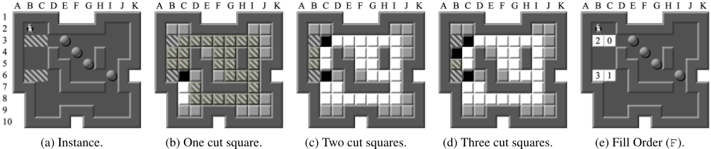
An instance of Sokoban has k movable blocks (stones) and k goal squares placed on a grid-square maze defined by immovable blocks (walls) and free squares. There is an additional block called the man which is the only block that can be moved directly. The man can traverse free squares and push (never pull) a stone to an adjacent free square. Figure 1a shows a stone at square 3E, a goal square at 3B, the man at square 2B and a wall at 1A. A solution is a sequence of actions that moves the k stones from their initial squares to the k goal squares and an optimal solution has the minimum number of pushes. The moves of the man are not counted. Note that square 9C is considered dead; once a stone is pushed there it can never reach a goal square.
Let Q be the set of free squares of an instance, G ✓ Q the set of goal squares and B the set of stones. A state u is a pair u = (p(B)↪m), where p is a map from the stones to the free squares and m is the position of the man. For a stone at square p(b) let δ(p(b)↪ g) be the minimum cost to push the stone at p(b) to square g when the man is at m in an instance with only one stone. This cost ignores all other stones. The enhanced minimum matching (EMM) is the standard heuristic of Sokoban, it is based on a minimum cost perfect matching in the complete bipartite graph between stones and goal squares with edge set ¶(b↪ g) ♣ b 2 B↪ g 2 G♦ and weights δ(p(b)↪ g). In this bipartite graph let M ⇤ be a minimum cost perfect matching. The matching cost is enhanced with linear conflicts that increase the heuristic value by two when a pair of adjacent stones is in the optimal path of each other, each stone can be part of only one linear conflict. Let L be the number of linear conflicts in a state. Then, the value of EMM for a state u is,
A series of articles [Pereira et al., 2013; 2014; 2015] introduced admissible PDB heuristics to Sokoban. The heuristic I [Pereira et al., 2015] provides the best previous results. It uses an instance decomposition to obtain an intermediate goal state. If all stones on a set of non-dead squares M have to pass over a fixed cut square c to be pushed to all reachable goal squares, the cut square c is used as an intermediate goal state. The squares in M are the maze zone squares and all other non-dead and non-goal squares are the goal zone squares. Figure 1b shows an instance decomposition: the cut square shown at 6C is part of the maze zone, the two maze zone squares at 7C and 8C and for example a goal zone square at 7D.
The heuristic I is the sum of the cost to solve two independent subproblems that are a relaxation of the original problem. The cut square defines the intermediate goal state and it can store many stones and the man simultaneously (this is the relaxation). The maze subproblem corresponds to the cost to push stones that are in the maze zone to the cut square. The goal subproblem corresponds to the cost to push stones at the cut square and in the goal zone to the goal squares. Let hM and hG be respectively the heuristic functions for the maze and goal subproblems. The value of heuristic I for a state u is defined as the sum of hM and hG.
A PDB is used to compute hM . The abstraction used maintains only k0 of all k stones in the instance, a PDB-k0 uses an abstraction of k0 stones. For this PDB, there is a unique abstract goal state that has k0 stones placed at the cut square. To build the PDB the algorithm performs a reverse search from the abstract goal state to enumerate all reachable abstract states with stones k0 in the maze zone. Let δ(p(P)) be the cost stored in the PDB for an abstract state u0 with stones P ✓ B. To compute hM the algorithm creates a partition B of all stones in the maze zone into parts P of size k0 . Among all possible partitions B the heuristic tries to find one that maximizes the heuristic value as described in [Pereira et al., 2015]. The value of hM for a state u is,
A modified state is used to compute hG. Stones in the maze zone are placed at the cut square and the position of the man is changed accordingly, all stones in the goal zone remain the same. A complete description of the procedure can be found in [Pereira et al., 2015]. Let d be this new map from the stones to free squares and position of the man. Let L be the number of linear conflicts in a state considering only stones in the goal zone and at the cut square. Finally, the value of hG for a state u is defined as,
In addition to the heuristic I, Pereira et al. [2015] introduced the tie-breaking rule called fill order F. It uses the property that there is an order to fill the goal squares respecting the restrictions of the instance. F attempts to approximate this order by placing all stones on goal squares and removing them in an arbitrary order with reverse moves. If a reverse move is possible the stone is removed from the instance and the corresponding goal square receives a priority value equal to the number of stones removed so far. This process continues until all stones have been removed. During the search, nodes with stones on goal squares with higher numbers are preferred. Figure 1e shows the order computed by F.
3 Proposed Pattern Database Heuristic based on Multiple Intermediate Goal States
In this section, we describe a simple method to extend the heuristic I to use multiple intermediate goal states and we show why it is ineffective. We present a more complex approach our novel admissible PDB heuristic D and describe how to compute the it efficiently in Section 3.2.
3.1 Instance Decomposition and Independent Subproblems
We want to find a set of cut squares C that maximizes the size of the maze zone M. To find such a set we analyze all possible sets of cut squares of fixed size. Given a set C we perform k reverse searches one for each goal square in which we place a single stone at the goal square. In all searches the squares in C are blocked for the stone, it cannot be placed at them. Then, all reachable non-dead and non-goal squares in these searches are part of the goal zone, and all other nondead squares are part of the maze zone. By construction, all stones in the set of non-dead squares M can only be pushed to the goal zone passing over the squares in C.
We place a number in front of the letter I (and later D) to define the number of cut squares used. 1I uses one cut square and 2I uses two cut squares. The PDB construction for heuristic I using more cut squares is the same as the original approach the only difference is that there are more abstract goal states. Each combinations of k0 stones on the cut squares generates an abstract goal state. With two cut squares, x stones on one cut square and y on the other, and k0 = 4 stones, we have five abstract goal states (x↪ y) = (0↪ 4)↪ (1↪ 3)↪ (2↪ 2)↪ (3↪ 1) and (4↪ 0). Each pair (x↪ y) is a unique abstract goal state. When computing hG for each stone in the maze zone, it is unknown which cut square will be used in pushing that stone into the goal zone. Then, when placing stones in the maze zone at the cut squares, the stone will be placed at the closest cut square for each goal square. The remainder of the heuristic computation is the same.
An instance decomposition of Figure 1a using one cut square, Figure 1b, finds a maze zone with three squares (6C, 7C and 8C). Because of that 1I and plain EMM have the same heuristic value of 27 for that instance. In an instance decomposition using two cut squares (Figure 1c), the maze zone comprises almost the whole instance, a three cut squares decomposition increases the maze zone by one square (Figure 1d). 2I with a PDB-k0 = 4 provides the optimal solution cost of 23 for the maze subproblem, where all stones are pushed to the cut square on 3C. When computing hG, two stones are placed at each cut square and the cost of this subproblem is two. 2I provides the heuristic value of 25 which is lower than plain EMM; because of that small difference, 2I expands 100 times more nodes to solve the instance.
The solution to improve the heuristic value is to solve the subproblems recognizing that they are dependent - the number of stones in each cut square in both subproblems has to be the same. We call this heuristic D. Using it in the instance shown in Figure 1a it provides the heuristic value of 31 - the optimum solution cost.
3.2 PDB Construction and Heuristic Computation
In heuristic D, we have a unique PDB for each abstract goal state generated by the combinations of k0 stones on the cut squares. One PDB for each pair (x↪ y) of the previous example. Let a be an assignment that maps stones in the maze zone to cut squares, stones in the goal zone remain the same. Let A be the set of all possible such assignments. Let δa(P)(p(P)) be the cost in one of the PDBs for an abstract state with subset of stones P, the number of stones in each cut squares defined by a(P) selects the PDB. To guarantee admissibility of heuristic D we have to find an assignment a that minimizes the sum of hM and hG. Thus, the value of heuristic D for a state u is defined as,
In the following, we describe how to compute the partition B and an optimal assignment efficiently.
Partitioning Computation
When computing B it is unknown at the time which cut square will be assigned to each stone. We assume that each subset P will be assigned to the set of cut squares that minimizes its cost and thus selecting the PDB with minimum cost. If k0 = 2, the optimal B can be found in polynomial time by a maximum weighted matching. If k0 > 2, we use a greedy randomized constructive method based on the one proposed by [Pereira et al., 2015]. The method starts by querying the cost of every subset, all ( k k0 ) subsets. Then, it ranks the subset according to the number of conflict pushes: the difference between the cost of the subset and the cost to push each stone in the subset individually to its closest cut square. Then, a greedy randomized method selects a disjoint partition trying to maximize the sum of the conflict pushes. Only subsets with all stones in the maze zone are included in B.
Assignment Computation
The assignment computation, in general, is the costly part of the heuristic. If the sum of conflict pushes in B is zero, we return the value of EMM. We only assign cut squares for stones in parts P with conflict pushes greater than zero, all other parts are removed from B. The intuition is that we just have to select cut squares for stones that are likely to increase the heuristic value. The simplest approach is to compute the cost of all possible assignments. When checking all possible assignments we call the heuristic the exhaustive heuristic DE .
The difficulty is that the number of stones in B could be k and thus, we have to check the cost of ♣C♣k assignments for a single state. To find an optimal assignment more efficiently we propose the use of a branch and bound computation.
We use a best-first branch and bound computation (BB). At each step in the BB a stone is assigned to a cut square. At the beginning, no stones have cut squares assigned and thus the lower bound is equal to EMM. If all stones in a part have cut squares then we compute the lower bound, otherwise, we just use the lower bound of the parent in the BB tree. The lower bound is defined as the cost of the two subproblems, but only parts where all stones have assigned cut squares use the cost of the PDB. The upper bound is defined as the cost of EMM plus the number of conflict pushes. The heuristic D using the BB is called DB .
3.3 Admissibility
In this subsection, we show that the heuristic D is admissible. Let h⇤ be the perfect heuristic. It is witnessed by some optimal sequence of actions S. For each stone in any part of B, consider the corresponding subsequence of S that brings it for the first time to some cut square. Such a subsequence must exist, by definition of the cut squares. The final position of each stone in these subsequences defines an assignment a of the stones in B to the cut squares. For all the stones in B, there must be a subsequence disjoint from the subsequence above, that brings it from the cut square to some goal square. Similarly, for all remaining stones there must be such a sequence. These subsequences define a matching M of stones to goal squares. Therefore, we have a pair (a↪M) and the value of h⇤ can be defined as h⇤ (a↪ M) = δ(p(B)↪ a(B)) + δ(a(B)↪ M(B)). Let hD (a⇤ ↪ M ⇤ ) = hM (p(B)↪ a⇤ (B)) + hG(a⇤ (B)↪ M ⇤ (B)) be the heuristic D with an optimal assignment a⇤ that minimizes the total cost given an optimal matching M ⇤ .
Proof. For any state, we want to show that hD (a⇤ ↪M ⇤ ) h⇤ (a↪ M).
By definition, the pair (a⇤ ↪M ⇤ ) minimizes the value of hD , any other pair (a↪M) cannot provide a lower value. Thus, we have that hD (a⇤ ↪M ⇤ ) hD (a↪M).
Now, we want to show that hD (a↪M) h⇤ (a↪M) where (a↪M) is the pair extracted from the optimal sequence S. First, consider hM and δ(p(B)↪ a(B)) both heuristics compute the cost to push the same set of stones from their original squares p(B) to the same set of cut squares a(B). The value of δ(p(B)↪ a(B)) accounts for conflicts between all stones in B, but the value of hM accounts only for conflicts that occur within each part P and thus it must be a lower bound on δ(p(B)↪ a(B)). A similar argument also applies for δ(a(B)↪M(B)) and hG. All stones B have the same original a(B) and destination M(B) squares. The value of hG accounts only for linear conflicts while δ(a(B)↪M(B)) accounts for all conflicts which include linear conflicts. Thus, hG must be a lower bound on δ(a(B)↪M(B)). Therefore,
4 Tie-Breaking Rule
Having the f-value equal to the optimal solution length does not necessarily mean a solution is close at hand; there can be a prohibitively large number of states remaining to be expanded. This makes tie-breaking rules important. When comparing two Sokoban states, the one with more stones on goal squares, in general, is closer to being solved. Moreover, there is an optimal order to place stones on goal squares such that a solution can be found or the solution cost is minimized. The tie-breaking rule F [Pereira et al., 2015] explores these ideas to speed up the process of finding solutions. Using F the search expands fewer nodes and solves more instances, but it has three main sources of errors: the total order of the goal squares, the rule used to define the order, and the assignment of partial priorities.
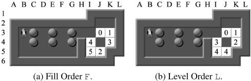
A total order may be attempting too much. When there is insufficient information to define an order to fill the goal squares one should not be preferred to the other. Figure 2a shows an order defined by F. In this instance according to the rule F, the goal square with number three has to receive a stone before the goal square with number two, which is not a feasible solution and thus the order is wrong. The rule used to define the order could be strengthened to avoid this type of error. Also, giving partial priorities may prioritize nodes with stones on goal squares with lower priorities such that those with higher priorities cannot be filled anymore. These problems may cause the search to explore a large portion of the search space without finding a solution.
To solve these problems we propose the tie-breaking rule level order (L). We compute L by placing all stones on goal squares. Then, iteratively we remove a stone with reverse moves. A stone is considered removed if it can reach a square that has a stone on it on the initial state of the instance without moving other stones on goal squares. Goal squares that have their stones removed in the same iteration receive the same priority. If after one iteration no stone can be removed, all the remaining goal squares with stones receive the highest priority. Figure 2b shows the order defined by L. During the search, a node receives a priority of the goal square with a stone only if all the goal squares with higher priority (bigger numbers) already have stones. For example, (a) a node with a single stone on a goal square with priority three will not receive any priority, and (b) a node with two stones on goal squares with priority four and one stone on goal square with priority zero will receive a priority of two.
| # | 1I | 2I | 2D | UB | # | 1I | 2I | 2D | UB | # | 1I | 2I | 2D | UB | # | 1I | 2I | 2D | UB |
|---|---|---|---|---|---|---|---|---|---|---|---|---|---|---|---|---|---|---|---|
| 1 | 97 | 93 | 97 | 97 | 24 | 518 | 517 | 534 | 544 | 47 | 201 | 183 | 201 | 209 | 70 | 329 | 327 | 329 | 333 |
| 2 | 131 | 123 | 131 | 131 | 25 | 378 | 361 | 378 | 386 | 48 | 200 | 186 | 200 | 200 | 71 | 298 | 300 | 302 | 308 |
| 3 | 134 | 126 | 134 | 134 | 26 | 175 | 162 | 175 | 195 | 49 | 106 | 88 | 114 | 124 | 72 | 294 | 262 | 294 | 296 |
| 4 | 355 | 343 | 355 | 355 | 27 | 359 | 350 | 359 | 363 | 50 | 102 | 100 | 100 | 370 | 73 | 441 | 437 | 441 | 441 |
| 5 | 141 | 133 | 141 | 143 | 28 | 290 | 287 | 290 | 308 | 51 | 118 | 100 | 118 | 118 | 74 | 182 | 176 | 190 | 212 |
| 6 | 106 | 100 | 106 | 110 | 29 | 132 | 130 | 132 | 164 | 52 | 379 | 359 | 379 | 421 | 75 | 263 | 267 | 273 | 295 |
| 7 | 80 | 86 | 86 | 88 | 30 | 407 | 400 | 407 | 465 | 53 | 186 | 182 | 186 | 186 | 76 | 194 | 196 | 198 | 204 |
| 8 | 220 | 220 | 220 | 230 | 31 | 236 | 233 | 236 | 250 | 54 | 181 | 178 | 181 | 187 | 77 | 360 | 238 | 364 | 368 |
| 9 | 231 | 222 | 231 | 237 | 32 | 115 | 122 | 129 | 139 | 55 | 120 | 115 | 120 | 120 | 78 | 136 | 136 | 136 | 136 |
| 10 | 510 | 510 | 510 | 512 | 33 | 152 | 140 | 170 | 174 | 56 | 193 | 193 | 201 | 203 | 79 | 170 | 149 | 170 | 174 |
| 11 | 213 | 209 | 213 | 241 | 34 | 164 | 164 | 164 | 168 | 57 | 217 | 219 | 219 | 225 | 80 | 231 | 201 | 231 | 231 |
| 12 | 206 | 198 | 208 | 212 | 35 | 368 | 352 | 368 | 378 | 58 | 197 | 189 | 197 | 199 | 81 | 167 | 141 | 173 | 173 |
| 13 | 224 | 224 | 224 | 238 | 36 | 511 | 502 | 511 | 521 | 59 | 218 | 222 | 222 | 230 | 82 | 137 | 131 | 137 | 143 |
| 14 | 231 | 231 | 231 | 239 | 37 | 242 | 225 | 246 | 284 | 60 | 148 | 147 | 150 | 152 | 83 | 194 | 184 | 194 | 194 |
| 15 | 100 | 106 | 108 | 122 | 38 | 79 | 79 | 79 | 81 | 61 | 253 | 255 | 255 | 263 | 84 | 153 | 149 | 155 | 155 |
| 16 | 170 | 162 | 170 | 186 | 39 | 658 | 598 | 658 | 672 | 62 | 241 | 236 | 241 | 245 | 85 | 307 | 307 | 307 | 329 |
| 213 | 314 | 324 | 63 | 429 | 424 | 429 | 431 | 86 | 124 | 112 | 124 | 134 | |||||||
| 17 | 203 | 199 | 203 | 124 | 40 | 314 | 306 | 237 | 381 | 385 | 87 | 223 | 217 | 223 | |||||
| 18 | 106 | 103 | 106 | 41 | 227 | 227 | 227 | 64 | 381 | 373 | 211 | 88 | 233 | ||||||
| 19 | 286 | 278 | 286 | 302 | 42 | 208 | 204 | 208 | 218 | 65 | 207 | 203 | 207 | 342 | 336 | 342 | 390 | ||
| 20 | 450 | 374 | 450 | 462 | 43 | 138 | 130 | 138 | 146 | 66 | 193 | 193 | 193 | 325 | 89 | 361 | 351 | 361 | 379 |
| 21 | 137 | 126 | 137 | 147 | 44 | 169 | 165 | 169 | 179 | 67 | 395 | 392 | 395 | 401 | 90 | 446 | 447 | 448 | 460 |
| 22 | 308 | 307 | 310 | 324 | 45 | 290 | 282 | 290 | 300 | 68 | 333 | 329 | 333 | 341 | |||||
| 23 | 432 | 428 | 432 | 448 | 46 | 227 | 217 | 227 | 247 | 69 | 223 | 217 | 223 | 433 |
5 Experimental Results
In this section, we compare our proposed heuristic D and tiebreaking rule L with the state-of-the-art heuristic I and tiebreaking rule F. As well, we include extending heuristic I to multiple intermediate goal states. All experiments were run on a PC with an AMD FX-8150 CPU running at 3▷6 GHz with 32 GB of RAM. We use the standard limits for Sokoban of 20 million expanded nodes or one hour of CPU time. In our experiments a search ended either because a solution was found or the time limit was reached, the node limit was never reached. The standard test set xSokoban of 90 instances is used.
5.1 Instance Decomposition and PDB Construction
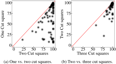
Our first experiment is regarding instance decomposition. We compare the percentage of maze zone squares obtained by one, two, and three cut squares. These results are shown in Figure 3. Over the 90 instances, decompositions with one, two, and three cut squares on average include respectively 66%, 92% and 97% of the squares in the instance are maze zone squares. Using two cut squares has 100% of the maze zone squares in 33 instances, while using one cut has only three instances.
A two cut squares decomposition provides a considerable improvement in the percentage of maze zone squares over one cut square. Because of that we perform experiments to at most two cut squares. PDBs built with k0 = 4 are the largest that can be built for all instances in one hour, and previously provided the best results. Thus, we fix the size of k0 = 4 in all our experiments. On average, PDB-4 for 2I has 323↪ 572 entries and takes 15 seconds to build, while 2D has 695↪ 606 entries and takes 108 seconds.
5.2 Heuristics on Initial States and Proved Optimal Solutions
Table 1 shows the heuristic values for the initial states of the 90 instances. Column UB shows the best-known upper bound. The first information to be noted is that heuristic I when extended from one cut square 1I to two cut squares 2I has worse results in general, but it is still able to increase the heuristic value on some instances (e.g. #7). 2D improves the heuristic value on average by 1▷71 compared to 1I over instances where 1I doesn't provide the best-known solution. For some instances it may be hard to improve the heuristic value. For example, consider #10: the heuristic has not improved, but 1I has 32% maze zone squares while 2D has 100%. Thus during the search 2D will detect more deadlocks. 2D improves the heuristic value in 25% of the instances compared to 1I, including an enormous improvement of 18 for instance #33.
Highlighted entries in Table 1 are the instances for which the optimal solution cost is now known. If the heuristic value of the initial state or the lowest f-value on the open list when the time limit is reached is equal to the best-known solution, then the optimal solution length is known. Considering only the heuristic value for the initial states 14 instances have the optimal solution proved. 1I, 2I and 2D prove respectively 12, 1 and 14. The ones proved by 1I and 2I are a subset of 2D. Considering the f-value when the time limit is reached, 32 instances have their optimal solution cost proven. 2DB proves 32, and 1I proves 25, a subset of 2DB . For some instances, we may not prove the optimality of the solution cost because the upper bound is loose (best human solution). However, we can compare which heuristic is closer to solve the instance: over all algorithms, 1I has the highest or equal highest f-value on the open list at the end of the search for 64 instances while 2DB has it for 87 instances.
5.3 Solved Instances
All methods use the same basic code infrastructure and an A⇤ search. We applied an additional improvement to heuristic I to make the comparison fairer: only use the cost in the PDB if the whole subset of stones is in the maze zone. Doing this 1I can solve one more instance.
Table 2 shows all instances solved by at least one of the methods. We use two combinations of tie-breaking rules: IF corresponds to the previous best tie-breaking rule using inertia [Junghanns and Schaeffer, 2001] as first order rule, and fill order as second order rule, and LI corresponds to our proposed tie-breaking rule L as first level rule, and inertia as second order rule. For each heuristic (1I, 2I, 2DE , 2DB ) there are two columns, one for each tie-breaking rule (IF, LI). A dot in a specific column indicates that the instance defining the row was solved by that combination of heuristic and tiebreaking rule. With the exception of 2I all heuristics solve more instances using LI. The improvement is more significant in 2DB solving five more instances, but even 1I benefits from LI. For example in instance #21 it expands 100 times fewer nodes and reduces the time by more than half an hour.
Comparing the heuristics, 2I can only solve five instances, showing that the extension to multiple intermediate goal states is ineffective with heuristic I. Even with a more accurate heuristic, 2DE cannot solve more instances than 1I due to the cost of expanding nodes. 2DB can solve more instances than 1I with both tie-breaking rules. In computing Table 2, 2DB on average expands 10 times fewer nodes per second than 1I, but it solves seven more instances. In large search spaces the comparison of 1I and 2DB indicates that a heuristic that is more informed can be beneficial, even if more computationally expensive. Another point highlighted by the results of 2DB is the effort to prove the optimality and to find the solution. 2DB can prove the optimality of 32 instances. However, it can only find the optimal solution for 28.
| # | 1I | 2I | 2DE | 2DB | ||||
|---|---|---|---|---|---|---|---|---|
| IF | LI | IF | LI | IF | LI | IF | LI | |
| 1 | ÷ | ÷ | ÷ | ÷ | ÷ | ÷ | ÷ | ÷ |
| 2 | ÷ | ÷ | ÷ | ÷ | ÷ | ÷ | ||
| 3 | ÷ | ÷ | ÷ | ÷ | ÷ | ÷ | ||
| 4 | ÷ | ÷ | ÷ | ÷ | ÷ | ÷ | ||
| 5 | ÷ | ÷ | ÷ | ÷ | ÷ | ÷ | ||
| 6 | ÷ | ÷ | ÷ | ÷ | ÷ | ÷ | ||
| 7 | ÷ | ÷ | ÷ | ÷ | ÷ | ÷ | ÷ | ÷ |
| 9 | ÷ | ÷ | ÷ | ÷ | ÷ | ÷ | ||
| 17 | ÷ | ÷ | ÷ | ÷ | ÷ | ÷ | ÷ | ÷ |
| 21 | ÷ | ÷ | ÷ | ÷ | ||||
| 33 | ÷ | |||||||
| 38 | ÷ | ÷ | ÷ | ÷ | ÷ | ÷ | ÷ | ÷ |
| 43 | ÷ | ÷ | ÷ | ÷ | ÷ | ÷ | ||
| 48 | ÷ | ÷ | ||||||
| 51 | ÷ | ÷ | ÷ | |||||
| 53 | ÷ | ÷ | ÷ | ÷ | ÷ | ÷ | ||
| 55 | ÷ | ÷ | ÷ | |||||
| 57 | ÷ | |||||||
| 60 | ÷ | |||||||
| 65 | ÷ | ÷ | ÷ | ÷ | ÷ | ÷ | ||
| 73 | ÷ | ÷ | ÷ | ÷ | ÷ | ÷ | ||
| 78 | ÷ | ÷ | ÷ | ÷ | ÷ | ÷ | ÷ | ÷ |
| 79 | ÷ | ÷ | ÷ | ÷ | ÷ | ÷ | ||
| 80 | ÷ | ÷ | ÷ | ÷ | ÷ | ÷ | ||
| 81 | ÷ | ÷ | ÷ | ÷ | ||||
| 82 | ÷ | ÷ | ÷ | ÷ | ÷ | ÷ | ||
| 83 | ÷ | ÷ | ÷ | ÷ | ÷ | ÷ | ||
| 84 | ÷ | ÷ | ||||||
| Tot. | 21 | 22 | 5 | 5 | 20 | 21 | 23 | 28 |
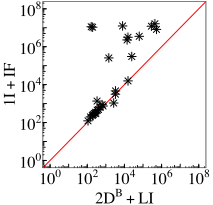
Figure 4 shows the detailed results of 1I+IF, the previous state-of-the-art, compared to 2DB +LI. 2DB uses at most 307 seconds more than 1I to solve any instance (#73). Comparing only the solved instances by both methods, 2DB uses more time in 13 instances while 1I uses more time in 15 instances. Regarding time, there is no clear winner. Regarding expanded nodes 2DB is the clear winner. Comparing only the solved instances by both methods 2DB expands 200 times fewer nodes on average.
6 Discussion
We have shown how to effectively apply PDB heuristics in transportation domains where the mapping of movable objects to goal locations is not fixed beforehand and where multiple intermediate goal states are helpful. We use our heuristic D and tie-breaking rule L and solve optimally more instances than previous methods. Domains like
- (a) Number of expanded nodes.
- (b) Total time in seconds.
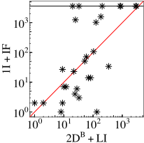
Figure 4: Comparison of the heuristics 1I+IF (previous state-of-the-art) and 2DB +LI.
ATOMIX [H¨uffner et al., 2001] and AIRPORT-IPC-4 [Trug et al., 2004] require D instead of heuristic I because in these domains the heuristic 1I in general doesn't provide maze zones with effective size. Tie-breaking rules inspired in L could also improve the results in these domains. Other domains with similar characteristics like STORAGE and TIDYBOT (both from IPC) are likely to benefit from our techniques.
The main limitation of our approach is that an increase of the number of cut squares will make the heuristic computation more costly. If the number of cut squares is similar to the number of goal locations the heuristic D is unlikely to improve the results. It is reasonable to increase the number of cut squares given that we are not using any specific method to prune the BB and that many selections of cut squares will not produce an optimal solution. In Sokoban for example, it is often the case that if more than one stone chooses the same cut square the solution is already infeasible. We could detect this infeasibility early without EMM. Pruning methods based on these cases could increase the efficiency of our method.
7 Conclusion
We extend the effectiveness of PDB heuristics in transportation domains and use this to increase the number of optimally solved instances of Sokoban. Further improvements in Sokoban could be produced by better strategies to select the subsets and by increasing the number of stones in the PDB. Another improvement could be related to the tie-breaking rule. We have proven the optimal solution cost for 32 instances, but we were not able to find a solution for four of them mainly because of tie-breaking.
Acknowledgments
The first author would like to thanks the financial support of CNPq.
@inproceedings{ijcai2016p100,
  title     = {Improved Heuristic and Tie-Breaking for Optimally Solving Sokoban},
  author    = {Pereira, André Grahl and Holte, Robert C. and Schaeffer, Jonathan and Buriol, Luciana S. and Ritt, Marcus},
  booktitle = {Proceedings of the Twenty-Fifth International Joint Conference on
               Artificial Intelligence, {IJCAI-16}},
  publisher = {AAAI Press / International Joint Conferences on Artificial Intelligence},
  editor    = {Subbarao Kambhampati},
  pages     = {662--667},
  year      = {2016},
  month     = {7},
  url       = {https://ijcai.org/proceedings/2016/100},
}
TY - CPAPER TI - Improved Heuristic and Tie-Breaking for Optimally Solving Sokoban AU - Pereira, André Grahl AU - Holte, Robert C. AU - Schaeffer, Jonathan AU - Buriol, Luciana S. AU - Ritt, Marcus T2 - Proceedings of the Twenty-Fifth International Joint Conference on Artificial Intelligence, IJCAI-16 PB - AAAI Press / International Joint Conferences on Artificial Intelligence PY - 2016 SP - 662 EP - 667 UR - https://ijcai.org/proceedings/2016/100 ER -Copied
Machine-readable versions of this paper, for tools and AI agents:





