Linear Arithmetic Satisfiability via Strategy Improvement

1 Introduction

Satisfiability modulo theories (SMT) solvers have proven to be extremely effective tools for solving a variety of problems. The traditional strength of SMT solvers has been in testing satisfiability of ground (quantifier-free) formulas, but many applications require quantifiers. For example, checking verification conditions for deductive verification [Ge et al., 2007], program synthesis [Solar-Lezama et al., 2006; Solar-Lezama, 2008; Reynolds et al., 2015], and model checking of array programs [Ghilardi and Ranise, 2010] all make use of quantifiers.

Integrating support for quantifiers into SMT solvers has been a long standing challenge. For theories that admit quantifier elimination, such as linear rational arithmetic (LRA), one option is to eliminate quantifiers and then apply an SMT solver to the resulting ground formula. However, for applications that require only a yes or no answer to the satisfiability problem, quantifier elimination is a computationally expensive and unnecessary step. Heuristic quantifier instantiation is a practical alternative to quantifier elimination [De Moura and Bjørner, 2007; Ge et al., 2007], but

Zachary Kincaid

Princeton University zkincaid@cs.princeton.edu

it is incomplete and may return unknown on difficult problem instances. First-order theorem provers (such as Vampire [Kov´acs and Voronkov, 2013] and E [Schulz, 2013]) are well-tuned for solving quantified formulas, but have limited support for reasoning modulo theories.

This article presents a novel procedure for checking satisfiability of (quantified) LRA formulas. As with some approaches to Quantified Boolean Formulas [Zhang, 2006; Janota et al., 2012], the procedure takes intuition from gametheoretical semantics of quantifiers [Hintikka, 1982]. We interpret a quantified formula as a game played by two players, SAT and UNSAT, whose goals are to prove that the formula is satisfiable and unsatisfiable, respectively. The players take turns instantiating quantifiers in the formula, with the existential quantifiers corresponding to moves of the SAT player and universal quantifiers corresponding to moves of the UNSAT player. SAT wins the game if the choices made by the players results in a model of the remainder of the formula (after all quantifiers have been instantiated); otherwise, UNSAT wins. A quantified formula is satisfiable if and only if there is a winning strategy for the SAT player; that is, if SAT has a way to win the game no matter how UNSAT plays.

The decision procedure proposed in this paper is based on synthesizing a winning strategy for one of the two players. The algorithm operates by iteratively improving the strategies for both players. At each step of the algorithm, one of the players proposes a candidate strategy. If the candidate is a winning strategy, then the status of the formula is known and the algorithm terminates. If the candidate is not a winning strategy, then the opposing player synthesizes a counterstrategy to beat it. In the next round, the opposing player proposes a new strategy that beats all previous strategies, and the two players switch roles. The process continues until one of the players obtains a winning strategy.

The next section defines the terminology and notation used in the rest of the paper. In ∗ 3 we define strategy skeletons. Strategy skeletons are similar to classical strategies, but have an order structure: our LRA decision procedure searches for winning strategy skeletons by ascending in this ("improvement") order. ∗ 4 describes a procedure for constructing a counter-strategy to a candidate strategy skeleton. ∗ 5 presents the decision procedure for LRA. ∗ 6 discusses how to extend the strategy improvement procedure to other theories, in particular linear integer arithmetic. We present experimental re-

2 Game Semantics for Linear Arithmetic

The definitions that follow are mostly standard, but the reader who is unfamiliar with the game-theoretic interpretation of quantifiers in first-order logic may wish to read ∗ 2.2.

2.1 Linear Arithmetic

The syntax of linear rational arithmetic (LRA) is as follows. The set of terms is defined by the following grammar

where x is a variable symbol and c is a rational number. Ground formulas are defined by the grammar

Notice that we (without loss of generality) assume that formulas are negation-free. A prenex formula is a formula of the form

where each Qi is either 9 or 8, F is a ground formula, and all variable symbols ¶x1↪ ▷▷▷↪ xn♦ are assumed to be distinct. For a formula ', we use fv(') to denote the free variables which appear in '; similarly, fv(t) denotes the free variables of the term t. A prenex formula is a sentence if it has no free variables.

A valuation is a function M : V ! Q, where V is some finite set of variable symbols and Q denotes the set of rational numbers. For a term t and a valuation V , we use JtKM to denote the interpretation of t within the valuation M. We use M ♣= ' to denote that M satisfies the formula ' (M is a model of '), defined in the usual way. Many modern SMT solvers have the capability of computing satisfying valuations for satisfiable ground formulas [De Moura and Bjørner, 2008; Barrett et al., 2011; Dutertre, 2014].

For a valuation M, a variable x, and a rational number c, we use M¶x 7! c♦ to denote the extension of M where x is interpreted as c:

For a formula ', variable x, and term t, we use '[x 7! t] to denote the formula obtained from ' by substituting each free occurrence of x with t. For a sequence ⇡, we use ♣⇡♣ to denote the length of ⇡ and ⇡i to denote the ith element of ⇡.

2.2 Satisfiability Games

A prenex sentence

defines a satisfiability game, which is played as follows. There are two players, SAT and UNSAT, which take turns picking rational numbers. At round i of the game, if Qi is 9, then SAT chooses a rational number to assign to the variable xi; if Qi is 8, then the choice belongs to UNSAT. After playing this game for n rounds, the players' choices define a play ⇢ 2 Qn : a sequence of rational numbers of length n. This play can be identified with a valuation of the variables M ⇢ : ¶x1↪ ▷▷▷↪ xn♦ ! Q where for each i, M ⇢ (xi) , ⇢i. The SAT player wins ⇢ if M ⇢ ♣= F , otherwise UNSAT wins.

A strategy for a satisfiability game determines the next move for a player as a function of the sequence of previous moves in the game:

Definition 2.1 (Strategy). Let

be a prenex LRA sentence. A SAT strategy for the satisfiability game ' is a function

Similarly, an UNSAT strategy for ' is a function

We say that a play ⇢ of ' conforms to a SAT strategy f if for every i 2 ¶1↪ ▷▷▷↪ n♦ such that Qi is 9, we have

That is, ⇢i = f(⇢1▷▷▷⇢i-1) whenever f(⇢1▷▷▷⇢i-1) is defined. Similarly, a play ⇢ of ' conforms to an UNSAT strategy g if ⇢i = g(⇢1▷▷▷⇢i-1) whenever g(⇢1▷▷▷⇢i-1) is defined.

We say that a SAT strategy f is winning if SAT wins every play that conforms to f. Similarly, an UNSAT strategy g is winning if UNSAT wins every play that conforms to g. It is easy to show that ' is satisfiable if and only if the SAT player has a winning strategy of the satisfiability game for ' (and ' is unsatisfiable if and only if the UNSAT player has a winning strategy).

For any prenex sentence ', we use ≻' to refer to the negation-free formula equivalent to the negation of ', obtained in the usual way. The formula ≻' defines a dual game, which is played as ' but with the roles of the SAT and UNSAT player reversed. It is often useful to define terminology and algorithms for the SAT player and leave the analogous definition for the UNSAT player implicit by appealing to duality. For example, rather than defining UNSAT strategies explicitly, we could define an UNSAT strategy to be a SAT strategy for the dual game ≻'. Note that, due to the completeness of the theory of linear rational arithmetic, we have:

Proposition 2.2. Let ' be a prenex sentence. UNSAT has a winning strategy for ' if and only if SAT has a winning strategy for the dual game ≻'.

3 Strategy Skeletons

As defined in ∗ 2.2, a strategy is a function that determines the next move for a player starting from any position in the game. A strategy skeleton determines a finite set of possible moves for any position. A key feature of strategy skeletons (which are formally defined below) is that they are ordered: one skeleton is "better" than another if it associates more moves with every position. This order will be exploited by the strategy improvement algorithm in ∗ 5, that operates by proposing a sequence of increasingly "better" candidate strategy skeletons.

Definition 3.1 (Strategy Skeleton). Let

be a prenex LRA sentence. A SAT strategy skeleton for ' is a finite, non-empty set S ✓ (Term [ ¶÷♦)n of sequences over terms plus a distinguished placeholder ÷, where each sequence ⇡1· · · ⇡n 2 S has length n and such that for all i 2 ¶1↪ ▷▷▷↪ n♦,

• ÷ if Qi is 8, then ⇡i is ÷
• ÷ if Qi is 9, then ⇡i is a term and fv(⇡i) ✓ ¶x1↪ ▷▷▷↪ xi-1♦

An UNSAT strategy skeleton for ' is defined to be a SAT strategy skeleton for the dual game ≻'.

Example 3.2. Consider the following formula:

which is visualized as the tree to the right. This tree indicates the moves available to a SAT player who plays according to this skeleton: on turn 1, the SAT player must

One possible SAT strategy skeleton for ' is:¶1÷((x + 1)◁2)÷↪ 1÷(x + 2)÷♦ ↪

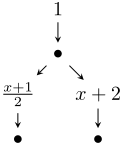
choose 1. On turn 2, the choice belongs to the UNSAT player (represented by the placeholder ÷). On turn 3, SAT may choose between (x+1)◁2 and x+2 (where x is the value the UNSAT player chose in the previous turn). Turn 4 again belongs to the UNSAT player, after which the game is finished.

÷

÷

Similar to the way that a strategy can be interpreted as a collection of plays (the plays that conform to that strategy), a strategy skeleton can be interpreted as a collection of strategies. We make this interpretation precise by defining what it means for a strategy to conform to a skeleton. Let ' = Q1x1▷Q2x2▷· · ·Qnxn▷F be a prenex LRA sentence, and let S be a strategy skeleton for the SAT player on '. We say that a play ⇢ of ' conforms to S if there exists some ⇡1· · · ⇡n 2 S such that for all i 2 ¶1↪ ▷▷▷↪ n♦ such that Qi is 9, we have JxiKM⇢ = J⇡iKM⇢ . We say that a strategy f for ' conforms to S if every play that conforms to f also conforms to S. A strategy skeleton is winning if some winning strategy conforms to it.

Winning formulas The goal of our decision procedure for LRA is to compute a winning skeleton for one of the players. The next step in developing this algorithm is to give a method for answering the question is a given candidate strategy skeleton winning? This question can be encoded into a universally quantified formula (the winning formula for the skeleton) which is satisfiable if and only if the skeleton is winning. The intuition behind this encoding is that we may replace each existential quantifier in the formula (representing the infinitely many possible moves available to the SAT player) with a finite disjunction (representing the finitely many possible moves that are available to the SAT if the play must conform to the given skeleton).

Formally, we define the winning formula win(S↪ ') for a strategy skeleton S for the game ' recursively as follows:

where we write S !t S0 iff S0 = ¶⇡ : t⇡ 2 S♦ and S0 is non-empty.

Proposition 3.3. Let ' be a formula and let S be a SAT strategy skeleton for '. There is a winning SAT strategy for the game ' that conforms to S if and only if win(S↪ ') is satisfiable.

Example 3.4. Again consider the formula ' and SAT strategy skeleton from Example 3.2. The winning formula is

One may check that the winning formula is satisfiable, and therefore the strategy skeleton is winning and ' is satisfiable.

4 Counter-strategies

If a given strategy skeleton is not winning, then the opposing player has a counter-strategy skeleton that beats it (that is, the counter-strategy wins against every strategy that conforms to the given skeleton). In this section, we formalize counterstrategies and give an algorithm for synthesizing them.

Given a formula ', a SAT strategy skeleton S for ', and an UNSAT strategy skeleton U for ', we say that U is a counterstrategy for S (U beats S) if there exists a strategy f that conforms to U such that every play that conforms to both S and f is a win for UNSAT. Counter-strategies for UNSAT strategy skeletons are defined similarly. We may observe the following:

Observation 4.1 (Anti-symmetry). Let S be a SAT strategy skeleton and U be an UNSAT strategy skeleton. It cannot be the case that S is a counter-strategy for U and U is a counterstrategy for S.

This kind of anti-symmetry is the key to our strategy improvement algorithm making progress. Throughout the course of the algorithm, SAT will propose a sequence of strategies S0↪ S1↪ ▷▷▷ and UNSAT will propose a sequence of strategies U0↪ U1↪ ▷▷▷, that are arranged as follows:

The inclusions S0 ✓ S1 ✓ ▷▷▷ (and U0 ✓ U1 ✓ ▷▷▷) hold by construction: Si+1 is defined to be the union of Si and a counter-strategy that beats Ui. Anti-symmetry ensures that the inclusions are strict, so that the players make progress towards a winning strategy.

We now consider the question of how counter-strategies may be synthesized. Given a formula ' and a SAT strategy S, Algorithm 1 either finds a counter-strategy to S or determines that no counter-strategy exists (that is, S is a winning strategy skeleton). (By duality, passing Algorithm 1 the formula ≻' and an UNSAT strategy U for ' finds a counter-strategy to U or determines that U is winning).

We explain Algorithm 1 by illustrating its operation on the formula from Example 3.2,

1 Procedure has-counter-strategy(S↪ ') Input : LRA sentence ' =Q1x1 · · ·Qnxn▷F, SAT strategy S Output: Counter-strategy to S if one exists; None if no counter-strategy exists /* Compute Herbrandized winning formula */ 2 for each ⇡ such that ⇡ ÷ ⇡0 2 S for some ⇡0 do 3 herbrand[⇡÷] fresh Herbrand constant 4 win false 5 for ⇡ 2 S do 6 G F 7 for i n downto 1 do 8 if Qi is 9 then 9 G G[xi 7! ⇡i] 10 else 11 G G[xi 7! herbrand[⇡1· · · ⇡i]] 12 win win _G /* win is the Herbrandized winning formula */ 13 if ≻win is satisfiable then /* Synthesize a counter-strategy for S */ 14 Let M ♣= ≻win 15 (U↪G) css('↪M↪ λx▷?↪ ✏↪ S) /* Alg. 2 */ 16 return Counter-strategy U 17 else /* S is a winning strategy */ 18 return None

using the SAT strategy S = ¶0÷x÷↪ 0÷(2x)÷♦ for '. Following the definition of win from the previous section, the winning formula for S is as follows:

Algorithm 1 begins by computing a Herbrandization of this winning formula (replacing each universally quantified variable with a fresh constant symbol), so that witnesses for each quantified variable can be computed from a model of its negation (should a model exist). The auxiliary map herbrand keeps track of the symbols introduced by Herbrandization:

After lines 2-12, the Herbrandized winning formula win is:

Notice that there is only one Herbrand constant (x) corresponding to the variable x and there are two (z1 and z2 ) corresponding to the variable z. The intuition behind this can be illustrated by the structure of the satisfiability game tree for ' when the SAT player conforms to S, depicted to the right. The SAT player begins the game by playing

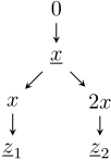
0 for w. The UNSAT player responds by choosing a value for x (which we call x). The SAT player then has a choice to play

1 Procedure css('↪M↪M ⇡ ↪ ⇡↪ S) Input : LRA formula ' =Qxi· · ·Qxn▷F, ValuationM : Image(herbrand) !Q ValuationM ⇡ : ¶x1↪ ▷▷▷↪ xi-1♦ !Q Path ⇡ 2 (Term [ ¶÷♦)i-1 SAT strategy S for ' Output: (U↪ G), where U is an UNSAT strategy G is a formula, and such that M ⇡ ♣= G, and For anyM 0 ♣= G, U beats S starting fromM 0 2 if i > n then 3 return (¶✏♦↪ ≻F ) 4 '0 Qi+1xi+1· · ·Qnxn▷F 5 if Qi is 8 then 6 M ⇡÷ M ⇡ ¶xi 7! Jherbrand[⇡÷]KM ♦ 7 S0 ¶⇡0 : ÷⇡0 2 S♦ 8 (U↪G) css('0 ↪M↪M ⇡÷ ↪ ⇡÷↪ S0 ) 9 t select(M ⇡÷ ↪ xi↪G) 10 return (¶t⇡ : ⇡ 2 U♦↪ G[xi 7! t]) 11 else 12 U ; 13 G true 14 for S !t S0 do 15 M ⇡t M ⇡ ¶xi 7! JtKM⇡ ♦ 16 (U +↪G+) css('0 ↪M↪M ⇡t ↪ ⇡t↪ S0 ) 17 G G^ (G+[xi 7! t]) 18 U U [U + 19 return (¶÷⇡ : ⇡ 2 U♦↪ G) Algorithm 2: Counter-strategy synthesis

either the same value that UNSAT played or twice that value. For each of these two moves, the UNSAT player may choose a different value for z: z1 corresponds to UNSAT's choice in the first case, and z2 corresponds to UNSAT's choice in the second.

After computing the Herbrandized winning formula win, Algorithm 1 checks if ≻win is satisfiable using an SMT solver. If ≻win is unsatisfiable then the procedure returns: win is satisfiable and so S is a winning strategy skeleton (by Proposition 3.3). Otherwise, the SMT solver returns a model of ≻win, say

The next step of Algorithm 1 is to use the model M to synthesize a counter-strategy skeleton for S that generalizes the strategy g, using Algorithm 2. Algorithm 2 traverses the satisfiability game tree pictured above: on the way down (traversing a path ⇡ from the root to a leaf), it builds a valuation (M ⇡ ) representing the unique play of the game where SAT conforms to ⇡ and UNSAT conforms to g. Since g beats S, this play is a win for UNSAT (i.e., M ⇡ ♣= ≻((y < 1 _ 2w <

y) ^ (z < y _ x < z))). For example, given the model M above the two paths in the example give the models:

When Algorithm 2 moves up the tree, it builds a counterstrategy skeleton U and a formula G such that:

• (i) The model corresponding to the unfinished play ⇡ is a model of G (i.e., M ⇡ ♣= G), and

Thus, at a recursive call of Algorithm 2 of depth i, U is a counter-strategy skeleton for S playing the part of the game after the ith quantifier (leaving the first i moves fixed as in M ⇡ ), and G is a formula that constrains the moves before the ith quantifier.

• (ii) U beats S starting from any play ⇢ such that M ⇢ ♣= G.

If depth i corresponds to an existential quantifier, then the counter-strategy is extended by prepending the placeholder value (line 18). If depth i corresponds to a universal quantifier in ', then Algorithm 2 uses a model-guided term selection function select to select an appropriate term with which to extend the counter-strategy (making conditions (i) and (ii) hold). ∗ 4.1 gives an implementation of select.

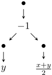
From property (ii) of Algorithm 2, we can conclude that when the call css('↪M↪ λx▷?↪ ✏↪ S) terminates, it returns a pair (U↪G) where U is a counter-strategy for S on the game ', and G is true. The final counter-strategy U that is synthesized by Algorithm 2 on this example is pictured to the right.

2

Finally, we summarize the preceding discussion in the following proposition:

Proposition 4.2. Let ' be a formula and let S be a strategy skeleton for '. If S is a winning strategy for ', then has-counter-strategy(S↪ ') returns None. If S is not winning, then has-counter-strategy(S↪ ') returns a strategy skeleton for the UNSAT player on ' that beats S.

4.1 Model-guided term selection

This sub-section defines select, the model-guided term selection procedure used in Algorithm 2. This function is inspired by model-based projection, an under-approximate quantifier elimination technique proposed in [Komuravelli et al., 2014], and the decision procedure for LRA presented in [Weispfenning, 1988] (a modification of the one proposed in [Ferrante and Rackoff, 1975]).

Given a ground formula F, a model M ♣= F, and a variable x 2 fv(F), the model-guided term selection function select(M↪ x↪ F) must find a term t such that x does not appear in t (fv(t) ✓ fv(F ) ∩ ¶x♦) and M ♣= F [x 7! t].

Observe that every atomic proposition in F that contains x can be written (after re-writing using standard arithmetical rules) in one of three forms: x = s, x < s, or s < x (where x does not appear in s). Let EQ(M↪ x↪ F) be the set of all terms s such that x = s appears in F and JxKM = JsKM , let UB(M↪ x↪ F ) be the set of all terms s such that x < s appears in F and JxKM < JsKM , and let LB(M↪ x↪ F) be the set of all terms s such that s < x appears in F and JsKM < JxKM . Since (by assumption) M is a model of F , M is also a model of F[x 7! t] for any term t such that t satisfies the same equations, lower bounds, and upper bounds as x (i.e., JtKM = JsKM for all s 2 EQ(M↪ x↪ F), JtKM < JsKM for all s 2

UB(M↪ x↪ F), and JsKM < JtKM for all s 2 LB(M↪ x↪ F)). The procedure select(M↪ x↪ F) proceeds as follows. If EQ(M↪ x↪ F) is non-empty, then we define eq(M↪ x↪ F) to be some arbitrarily-chosen member. Otherwise, suppose that UB(M↪ x↪ F) is non-empty. Then there exists a (not necessarily unique) least upper bound u 2 UB(M↪ x↪ F) such that JuKM  JsKM for all s 2 UB(M↪ x↪ F). We let lub(M↪ x↪ F) be an arbitrarily-chosen least upper bound for x if one exists. Similarly, we define glb(M↪ x↪ F ) to be an arbitrarily-chosen greatest lower bound if one exists. Finally, we define select: select(M↪ x↪ F ) ,

The term select(M↪ x↪ F) satisfies the same equations, lower bounds, and upper bounds as x. As a result, we have the following lemma, which is sufficient for the correctness argument of Algorithm 2 (in particular, the lemma is sufficient to prove that the algorithm maintains properties (i) and (ii) above):

Lemma 4.3 (Model preservation). Suppose M ♣= F. Then M ♣= F [x 7! select(M↪ x↪ F )].

The function select also satisfies a finite-image property, which is crucial for the termination argument of the decision procedure for LRA that we present in the next section:

Lemma 4.4 (Finite Image). Let F be a formula and x be a variable. The set ¶select(M↪ x↪ F) : M ♣= F♦ is finite.

Proof. Define an equivalence relation ⌘F on valuations, where M ⌘F M 0 if and only if M and M 0 satisfy the set of same atomic propositions in F. There are finitely many equivalence classes of ⌘F (since there are finitely many atomic propositions in F), and select selects equal terms for equivalent models, and so the set ¶select(M↪ x↪ F) : M ♣= F♦ is finite.

5 A strategy improvement algorithm for LRA

This section describes a decision procedure for linear rational arithmetic based on strategy improvement. The algorithm is given in Algorithm 3. Given an input formula

the algorithm operates as follows. First, query an SMT solver for a model of the formula F. If no model exists, then clearly ' is unsatisfiable. If a model does exist, then we may use it to construct an initial strategy skeleton for the SAT player, similarly to the way that Algorithm 2 constructs a counterstrategy from a model (lines 4-13).

Input : LRA sentence ' =Q1x1· · ·Qnxn▷F Output: true if ' is satisfiable, false if ' is unsatisfiable 1 if F is unsatisfiable then 2 return false /* Compute initial strategy for SAT */ 3 Let M ♣= F 4 G F 5 for i n downto 1 do 6 if Qi is 9 then 7 t select(M↪ xi↪G) 8 G G[xi 7! t] 9 ⇡i t 10 else 11 G G[xi 7! select(M↪ xi↪G)] 12 ⇡i ÷ 13 S ¶⇡1· · · ⇡n♦ 14 U ; /* Strategy improvement */ 15 while true do 16 switch has-counter-strategy(S↪ ') do 17 case Counter-strategy U 0 do 18 U U [U 0 19 otherwise do /* No counter strategy)S is winning */ 20 return true 21 switch has-counter-strategy(U↪ ≻') do 22 case Counter strategy S0 do 23 S S [S0 24 otherwise do 25 return false Algorithm 3: Satisfiability modulo LRA

After constructing the initial strategy skeleton to SAT, we begin the strategy improvement phase of the algorithm, depicted in Diagram . At the start of the loop, we have a SAT strategy skeleton S and an UNSAT strategy skeleton U, such that S beats U (or U is empty). First, we try to synthesize a counter-strategy to S. If counter-strategy synthesis fails, the algorithm terminates: S is a winning strategy, so ' is satisfiable. If has-counter-strategy does synthesize a counterstrategy, it is added to the candidate UNSAT strategy U (improving it). Next, we repeat this process for the candidate UNSAT strategy U, and either terminate upon proving that U is a winning strategy or find a counter-strategy with which to improve S and continue looping.

Algorithm 3 returns true only when it has synthesized a SAT strategy skeleton for which the winning formula is satisfiable (i.e., the negation of its winning formula is unsatisfiable), and returns false only when it has synthesized an UNSAT strategy skeleton for which the winning formula is satisfiable. Thus, partial correctness of Algorithm 3 is an immediate corollary of Proposition 3.3: if Algorithm 3 returns true, then ' is satisfiable, and if Algorithm 3 returns false, then ' is unsatisfiable.

The termination argument for Algorithm 3 is based on two properties: progress (as the algorithm progresses, the strategy skeleton S is strictly increasing), and finiteness (there is a finite bound on the size of S). The progress argument

(mentioned in ∗ 4) comes from the anti-symmetry property of counter-strategies (Observation 4.1). The finiteness argument is by induction on quantifier depth. The base case is by Lemma 4.4. If we assume that the finiteness condition holds for all strategies for a given formula ' of depth n, then we prove the same holds for depth n + 1 by arguing that the algorithm computes the first move of the game by calling select(M↪ x↪ F), where F is some formula obtained by substituting terms from a counter-strategy of depth n into a negated, Hebrandized winning formula of strategy of depth n, M is a model of F, and x is the variable associated with the first move of the game. By the induction hypothesis, the set of all possible such F is finite, so by Lemma 4.4, the set of terms that could be selected for x is finite, and thus the set of skeletons is finite.

Combining the above arguments for partial correctness and termination, we close the section with the following theorem:

Theorem 5.1. Algorithm 3 is a decision procedure for LRA.

6 Beyond LRA

The focus of this article is satisfiability in the theory of linear rational arithmetic, but the core ideas behind the strategy improvement algorithm can be extended to other theories. This section discusses what we require of a theory in order to apply our algorithm.

There are three assumptions on the theory that must be met in order to use strategy improvement as a decision procedure.

1. The quantifier-free fragment of the theory in question must be decidable, and models for satisfiable formulas must be effectively constructable.
2. The theory must be complete. This is required because Algorithm 3 checks that the (universally quantified) winning formula for a skeleton is satisfiable by checking that its (existentially quantified) negation is unsatisfiable.
3. The theory admits a model-guided term selection function that is model-preserving (Lemma 4.3) and has finite images (Lemma 4.4).

Thus, the design work involved in extending the strategy improvement algorithm to a new theory is in devising a term selection function. In fact, condition 3 can be weakened slightly to require only that a theory admits a modelguided virtual term selection function. A virtual term is a term that does not belong to the theory in question, but which may be evaluated in any model of the theory and for which substitution is theory-definable. Section 6.1 gives a term selection function (based on ideas from [Cooper, 1972; Komuravelli et al., 2014]) for linear integer arithmetic that makes use of such virtual terms.

Remark 6.1. It is worth noting that our requirements for virtual terms are stronger than ones usually employed by quantifier elimination procedures [Cooper, 1972; Loos and Weispfenning, 1993; Komuravelli et al., 2014; Bjørner and Janota, 2015]. For example, the LIA quantifier elimination procedure from [Cooper, 1972] makes use of the virtual term 1, which does not meet our requirements because it cannot be evaluated in the standard model of the integers.

We leave the development of term selection functions for other theories as a promising direction for future work.

6.1 Term selection for Linear Integer Arithmetic

Linear integer arithmetic is an important theory for application in program analysis and verification. The syntax of LIA is the same as for LRA, except that constants are integers, and the language is extended with divisibility predicates a♣t (where a 2 Z is a positive integer and t is a term). In the remainder of the section we will develop a virtual term selection function for linear integer arithmetic.

First we define virtual terms and virtual substitution. We consider virtual terms of the form bt◁ac + b, where t is a term with fv(t) ✓ fv(F) ∩ ¶x♦, a 2 Z is a positive integer, and b 2 Z is an integer. The syntax of LIA does not admit integral division bt◁ac, so virtual terms do not belong to the syntax of LIA. However, integral division can be interpreted in any valuation (Jbt◁acKM is well-defined), and for any formula ', variable x, and virtual term bt◁ac+b, we can perform a virtual substitution that yields a formula equivalent to '[x 7! bt◁ac + b] but which belongs to the syntax of LIA:

Definition 6.2 (Virtual Substitution). Let ' be a formula, x be a variable, and bt◁ac + b be a virtual term. Without loss of generality, we assume that every atomic proposition in ' in which x appears takes one of the following forms:

We define the virtual subsitution '[x bt◁ac + b] to be the formula obtained by renaming the bound variables in ' to avoid capture and replacing each atomic proposition in ' in which x appears as follows:

where s denotes a term with x ◁2 fv(s) and c and d denote positive integers. (Note that the equality symbol is not needed because s = s0 may be replaced by s < s0 + 1 ^ s0 < s + 1.)

The development of the previous three sections can be repeated with virtual terms and virtual subsitution in place of terms and classical substitution. The only thing that remains to extend the strategy improvement algorithm to LIA is to define a virtual term selection function vselect that satisfies the model preservation and finite image properties.

Let F be a LIA formula, let M ♣= F be a model, and let x be a variable. We require vselect(M↪ x↪ F) to satisfy the model preservation property

Since F is negation-free, it is sufficient for model preservation to hold on all the atomic propositions of F that contain x. Observe that every atomic propsition in F that contains x can be written in one of three forms: (cx < s), (s < cx), or (d♣cx + s) (where x does not appear in s). Let UB(M↪ x↪ F)

be the set of all atoms (cx < s) that appear in F such that cJxKM < JsKM , let LB(M↪ x↪ F) be the set of all atoms (s < cx) that appear in F such that JsKM < cJxKM , and let Div(M↪ x↪ F ) be the set of all divisibility atoms (d♣cx+s)

in F such that d divides Jcx + sKM . First we consider the constraints that the divisibility atoms Div(M↪ x↪ F) place on vselect(M↪ x↪ F). Let (d♣cx + s) 2 Div(M↪ x↪ F). Observe that for any integer z 2 Z,

() z ⌘ JxKM mod (d◁gcd(♣c♣↪ d)) Thus, the divisibility atom (d♣cx + s) is satisfied so long as

and require that

Jvselect(M↪ x↪ F)KM ⌘ JxKM mod ∆(M↪ x↪ F) ▷ Next, we consider the constraints that the upper bound atoms UB(M↪ x↪ F) place on vselect(M↪ x↪ F). Suppose that UB(M↪ x↪ F) is non-empty. Then there exists a term t, a positive integer a, and non-negative integer b less than ∆(M↪ x↪ F) such that:

1. (ax < t) 2 UB(M↪ x↪ F),

Jb(t - 1)◁ac - bKM  Jb(t0 - 1)◁a0 c - b0 KM . We define lub(M↪ x↪ F ) to be a virtual term b(t-1)◁ac-b satisfying these three properties (picking one arbitrarily if there are several choices). Property 2 ensures that lub(M↪ x↪ F) satisfies all divisibility constraints in Div(M↪ x↪ F ) and property 3 ensures that lub(M↪ x↪ F) satisfies all upper bound constraints UB(M↪ x↪ F). Property 2 and the fact that b is less than ∆(M↪ x↪ F ) implies that JxKM  Jlub(M↪ x↪ F )KM , and so lub(M↪ x↪ F ) also satisfies all lower bound constraints. However, if UB(M↪ x↪ F ) is empty, we need to consider lower bound constraints explicitly, so we define glb(M↪ x↪ F) analogously to glb(M↪ x↪ F) if LB(M↪ x↪ F) is non-empty. Finally, we define vselect:

1. Jb(t -1)◁ac - bKM ⌘ JxKM mod ∆(M↪ x↪ F), and 3. For any other t0 , a0 , b0 with the above properties, we have

vselect(M↪ x↪ F ) ,

JxKM mod ∆(M↪ x↪ F) otherwise The argument that the finite image property holds for vselect is the same as the one for select (Lemma 4.4).

7 Experimental Evaluation

We have implemented Algorithm 3 in a prototype tool called SIMSAT. The tool is implemented in OCaml and uses Z3 to solve ground formulas [De Moura and Bjørner, 2008].

Comparison with related techniques

Heuristic quantifier instantiation is a sound but incomplete technique that is commonly used to handle quantifiers in SMT solvers [De Moura and Bjørner, 2007; Ge et al., 2007]. Our

0.01

0.01

0.011

0.011

0.011

0.011

0.011

0.011

0.012

0.013

0.013

0.014

0.014

0.014

0.014

0.015

0.015

0.015

0.015

0.015

0.015

0.015

0.015

0.015

0.015

0.016

0.016

0.016

0.016

0.016

0.017

0.017

0.017

0.017

0.017

0.017

0.017

0.017

0.017

0.018

0.018

0.018

0.018

0.018

0.018

0.018

0.018

0.018

0.018

0.018

0.018

0.018

0.018

0.018

0.018

0.018

0.018

0.018

0.018

0

1,000

Instances Solved (easiest to hardest)

1729

1879

23

1

1

9

1

10

1

7

1

1

1

7

10

1

13

1

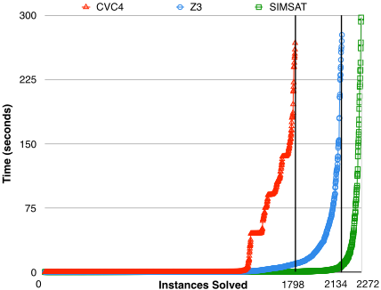
Figure 1: Distribution of run-time over solved instances 23

SIMSAT

Z3

CVC4

23

1

1

23

1

experimental evaluation compares with the experimental configuration of CVC4 [Barrett et al., 2011], which won the LRA category in the 2015 SMT competition. CVC4 uses a portfolio of quantifier instantiation techniques. 23 23 23 23

Time (seconds) 0 1 Instances Solved 1816 0 1401 1 Bjørner and Janota recently developed a decision procedure for LRA (as well as other theories) that is based on the intuition of satisfiability games [Bjørner and Janota, 2015]. Conceptually, their procedure solves satisfiability games by exploring the game tree in a forwards direction. The SAT and UNSAT player take turns instantiating quantifiers until one of them loses, and then backjumps to an earlier quantification level and learns a blocking clause to remove a part of the search space that will result in a loss for that player. In contrast, in Algorithm 3, players take turns synthesizing strategies for the entire game, rather than synthesizing the next move. Algorithm 3 requires solving larger formulas (corresponding to the whole game), but the payoff is a more "global" perspective of the game. 23 23 23 23 23 23 27 27 27 27 27 27 27 27 27

Dutertre developed an efficient algorithm for solving 9⇤8⇤ in the theory of linear rational arithmetic [Dutertre, 2015]. At a high level, Dutertre's algorithm operates similarly to Algorithm 3 when restricted to the 9⇤8⇤ fragment. Dutertre uses a term selection function similar to the one in ∗ 4.1, but with some interesing heuristic improvements (that do not extend to the case of arbitrary quantification in an obvious way). 27 27 27 27 27 27 27

Monniaux developed a lazy quantifier elimination algorithm for LRA formulas with alternating quantifiers that is based on geometric quantifier elimination (polyhedra projection) [Monniaux, 2010]. This algorithm was implemented in a satisfiability procedure in Z3 [Phan et al., 2012]. The experimental evaluation in [Bjørner and Janota, 2015] shows that Bjørner and Janota's algorithm outperforms lazy quantifier elimination, so we omit it from our evaluation.

Results

We evaluated SIMSAT on a suite of benchmarks drawn from SMT-LIB2 [Barrett et al., 2010] and Mjollnir [Monniaux, 2010]. The experimental evaluation was performed on a Linux machine with Intel Core i5 2.80GHz processors and 4GB of memory. The time limit was set to 300 seconds.

The table below summarizes the number of solved prob-

1

7

1

13

1

10

1

1

1

1

5

1

1

1

1

10

7

10

11

10

13

14

10

7

10

11

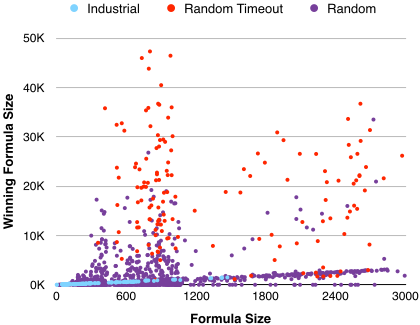
Table 1-1

359 8521

Figure 2: Formula size vs. Winning formula size

419 35806

Table 1-2

919 29477 585 31263 999 30140 959 93171 731 19675 981 46467 685 24583 961 33902 537 21732 791 35881 899 12209 795 43836 677 23848 801 15677 865 22758 935 28995 113 197 113 201 113 201 113 197 113 203 113 193 113 197 113 197 113 199 113 195 111 195 111 197 111 199 107 189 111 197 111 195 lem instances by each tool. The results are divided into three categories: industrial benchmarks (from SMT-LIB2) with an 9⇤8⇤ quantifier prefix, industrial benchmarks (from SMTLIB2) with a non-9⇤8⇤ quantifier prefix (all of which happened to have a quantifier prefix of the form 9⇤89), and random benchmarks (from both SMT-LIB2 and Mjollnir). SIMSAT, Z3 (implementing the algorithm from [Bjørner and Janota, 2015]), CVC4, and Yices (implementing the algorithm from [Dutertre, 2015]) all solve all industrial 9⇤8⇤ benchmarks (all tools have a mean running time of less than 0.01 seconds). On the remaining industrial benchmarks, SIMSAT and Z3 solve all instances (SIMSAT mean time 1 second, Z3 mean time 0.02 seconds) while CVC4 solves 83%. On the random benchmarks, SIMSAT dominates (93%), followed by Z3 (86%) and CVC4 (71%).

817 16097

111 201

791 52205	113 197 SIMSAT	Z3	CVC4	YICES
925 18676 Industrial 9⇤8⇤ (247)	113 197 247	247	247	247
957 22250 Industrial 9⇤89 (144)	113 199 144	144	119	-
525 16182 Random (2030)	113 197 1881	1743	1432	-

521 23754

113 201

875 36729 999 13319 923 14239 877 15679 109 187 109 189 113 197 113 201 The distribution of running times of the three tools across random benchmarks is depicted in the cactus plot in Figure 1 (a point (x↪ y) in the plot represents that x instances are solved in y seconds). Note that SIMSAT can solve in ⇠5.3s as many instances as Z3 can solve in 300s.

1 Figure 2 plots the size of input formulas against the size of the winning formula for the winning strategy computed by SIMSAT (or the last candidate strategy if SIMSAT did not terminate within 300 seconds). Formula size is measured as the number of nodes in a DAG representation of the formula. For legibility, the plot truncates input formula size at 3000 and the winning formula size at 50000. Note that on the industrial benchmarks, the relationship between input formula size and winning formula size is linear.

Linear integer arithmetic We also evaluated SIMSAT as a decision proecedure for linear integer arithmetic, using the virtual term selection procedure described in ∗ 6. The benchmarks are drawn from SMT-LIB2 and randomly generated benchmarks. The table below summarizes the number of solved problem instances by each tool (excluding Yices, which does not implement an LIA solver). SIMSAT and Z3 both solve all industrial instances (SIMSAT mean time 1.2 seconds, Z3 mean time 0.1 seconds), while CVC4 solves 59%. On the random benchmarks, SIMSAT solves the most instances (71%), followed by CVC4 (70%) and Z3 (58%).

	SIMSAT	Z3	CVC4
Industrial (390)	390	390	231
Random (300)	212	174	211

8 Conclusion

This article presents a decision procedure for the theory of linear arithmetic based on strategy improvement for satisfiability games. There are several avenues for future work in this direction. The strategy improvement algorithm is very sensitive to model selection, so it would be interesting to experiment with heuristics for different models of ground formulas. Another promising direction is to extend the strategy synthesis algorithm to other decidable theories, such as the theory of algebraic data types. Another direction is to investigate uses for the strategy synthesis capability of the algorithm: just as there are many applications for models of ground formulas, we believe there may be interesting uses for winning strategies of quantified formulas.