
Controllable Procedural Content Generation via Constrained Multi-Dimensional Markov Chain Sampling
Proceedings of the Twenty-Fifth International Joint Conference on Artificial Intelligence. Pages 780-785.
Abstract
Statistical models, such as Markov chains, have recently started to be studied for the purpose of Procedural Content Generation (PCG). A major problem with this approach is controlling the sampling process in order to obtain output satisfying some desired constraints. In this paper we present three approaches to constraining the content generated using multi-dimensional Markov chains: (1) a generate and test approach that simply resamples the content until the desired constraints are satisfied, (2) an approach that finds and resamples parts of the generated content that violate the constraints, and (3) an incremental method that checks for constraint violations during sampling. We test our approaches by generating maps for two classic video games, Super Mario Bros. and Kid Icarus.
- [Ching et al., 2013] Wai-Ki Ching, Ximin Huang, Michael K Ng, and Tak-Kuen Siu. Higher-order markov chains. In Markov Chains, pages 141-176.
- [Dahlskog et al., 2014] Steve Dahlskog, Julian Togelius, and Mark J Nelson. Linear levels through n-grams. Proceed- ings of the 18th International Academic MindTrek, 2014.
- [Guzdial and Riedl, 2015] Mathew Guzdial and Mark Riedl. Toward game level generation from gameplay videos. In FDG 2015, 2015.
- [Markov, 1971] Andrey Markov. Extension of the limit theo- rems of probability theory to a sum of variables connected in a chain. In Dynamic Probabilistic Systems: Vol. 1: Markov Models, pages 552-577. Wiley, 1971.
- [Mawhorter and Mateas, 2010] Peter Mawhorter and Michael Mateas. Procedural level generation using occupancy-regulated extension. In Computational Intel- ligence and Games (CIG), 2010 IEEE Symposium on, pages 351-358. IEEE, 2010.
- [Pachet and Roy, 2011] Franc ¸ois Pachet and Pierre Roy. Markov constraints: steerable generation of markov se- quences. Constraints, 16(2):148-172, 2011.
- [Shaker et al., 2011] Noor Shaker, Julian Togelius, Geor- gios N Yannakakis, Ben Weber, Tomoyuki Shimizu, Tomonori Hashiyama, Nathan Sorenson, Philippe Pasquier, Peter Mawhorter, Glen Takahashi, et al. The 2010 mario AI championship: Level generation track. TCIAIG, IEEE Transactions on, 3(4):332-347, 2011.
- [Shaker et al., 2015] Noor Shaker, Julian Togelius, and Mark J. Nelson. Procedural Content Generation in Games: A Textbook and an Overview of Current Research. Springer, 2015.
- [Smith and Mateas, 2011] Adam M Smith and Michael Mateas. Answer set programming for procedural con- tent generation: A design space approach. Computa- tional Intelligence and AI in Games, IEEE Transactions on, 3(3):187-200, 2011.
- [Smith and Whitehead, 2010] Gillian Smith and Jim White- head. Analyzing the expressive range of a level generator. In Proceedings of the 2010 Workshop on Procedural Con- tent Generation in Games, page 4. ACM, 2010.
- [Smith et al., 2009] Gillian Smith, Mike Treanor, Jim White- head, and Michael Mateas. Rhythm-based level generation for 2D platformers. In Proceedings of the 4th International Conference on Foundations of Digital Games, pages 175- 182. ACM, 2009.
- [Snodgrass and Ontañón, 2014] Sam Snodgrass and Santi- ago Ontañón. Experiments in map generation using markov chains. In FDG 2014, 2014.
- [Summerville et al., 2015] Adam James Summerville, Shweta Philip, and Michael Mateas. Mcmcts pcg 4 smb: Monte carlo tree search to guide platformer level gener- ation. In Eleventh Artificial Intelligence and Interactive Digital Entertainment Conference, 2015.
- [Togelius et al., 2013] Julian Togelius, Alex J Champandard, Pier Luca Lanzi, Michael Mateas, Ana Paiva, Mike Preuss, Kenneth O Stanley, Simon M Lucas, Michael Mateas, and Mike Preuss. Procedural content generation: Goals, chal- lenges and actionable steps. Artificial and Computational Intelligence in Games, 6:61-75, 2013.
References were extracted automatically from the PDF and may contain errors.
Full text extracted automatically from the PDF; figures, tables and equations may differ. The PDF is the version of record.
1 Introduction
Procedural content generation (PCG) studies the generation of content (e.g., textures, maps, quests, stories, etc.) algorithmically, allowing players to experience new and unique content. Recently there has been increased interest in using statistical approaches to model and produce video game maps [Dahlskog et al., 2014; Guzdial and Riedl, 2015].
In previous work [Snodgrass and Onta˜n´on, 2014] we introduced an approach using multi-dimensional Markov chains (MdMCs) which learned a statistical model from a set of training maps that could then be used to sample new maps with the same statistical properties. The main drawback of statistical approaches is that they do not provide the user much control over the output. In this paper, we describe three algorithms that, when paired with a probabilistic sampling approach, offer the user control over the properties of the output maps. Notice, however, that in addition to PCG the proposed algorithms generalize to other domains where (multi-dimensional) Markov chains are used to sample content (e.g., texture synthesis or music generation).
There has been work in constraining Markov models in order to steer the sampling process [Pachet and Roy, 2011] where the problem is formulated as a branch and bound problem searching over the set of sequences satisfying a set of constraints, and using variations on the log likelihood of the sequence as cost functions. The key differences with the work presented in this paper are that (1) we focus on multidimensional sequences (video game maps), instead of onedimensional sequences, and (2) we focus on sampling largescale sequences, which would be infeasible with the branchand-bound approach. Therefore, we employ larger section sizes to avoid the combinatorial increase in the search space.
The remainder of this paper is organized as follows. We start by specifically formulating the problem we try to address. After that, Section 2 provides some background on PCG and Markov chain-based map generation. Section 3 presents the proposed algorithms for constrained sampling on MdMCs, and Section 4 presents our experimental evaluation.
1.1 Problem Statement
The problem we are addressing in this paper is that of controllability in PCG algorithms based on statistical models, such as Markov chains. Currently, users are only able to control the output of a statistical generator by changing the training data or model configuration, both of which are unintuitive and ineffective methods when trying to produce maps with specific characteristics. To address this problem, we propose three constrained sampling algorithms that allow the user to define specific constraints to be enforced in the output maps.
2 Background
2.1 Procedural Map Generation
Procedural content generation (PCG) studies the algorithmic creation of content [Shaker et al., 2015], typically for video games. This section discusses statistical and constraint-based techniques for level generation.
We are interested in generators that learn statistical properties from training data (i.e., existing maps), and use them to sample new maps. Some interesting work in this area includes sampling new maps using n-grams trained on input maps [Dahlskog et al., 2014], as well as generating maps using a statistical model trained on gameplay footage [Guzdial and Riedl, 2015]. For testing our approach, we use the multidimensional Markov chain (MdMC) generator developed in our previous work [Snodgrass and Onta˜n´on, 2014].
We are also interested in techniques that produce outputs satisfying defined constraints. For example, Smith and Mateas [Smith and Mateas, 2011] describe an answer set programming approach to level generation. However, their approach produces levels satisfying the provided constraints using search, whereas our approaches aim to satisfy constraints while adhering to an underlying probability distribution.
In addition to the above approaches, many other level generation approaches have been put forward. For example, Smith et al. experimented with a rhythm-based approach [Smith et al., 2009], and Mawhorter and Mateas [Mawhorter and Mateas, 2010] explored using occupancy-regulated extension, a geometry assembly approach. There have even been level generation competitions [Shaker et al., 2011].
2.2 Markov-chain-basedMap Generation
In this section we give a brief introduction to multidimensional Markov chains (MdMCs). We then discuss how they are used to model training maps and sample new maps.
Markov Chains
Markov chains [Markov, 1971] model stochastic transitions between states over time. A Markov chain is defined as a set of states S = ¶s1↪ s2↪ ▷▷▷↪ sn♦ and the conditional probability distribution (CPD) P(St♣St-1), representing the probability of transitioning to a state St 2 S given that the previous state was St-1 2 S. The set of previous states that influence the CPD are referred to as the network structure of the model.
Higher-order Markov chains allow the network structure to include d 2 N previous states [Ching et al., 2013]. The CPD defining an order d Markov chain can be written as P(St♣St-1↪ ▷▷▷↪ St-d). That is, P is the conditional probability of transitioning to a state St, given the past d states.
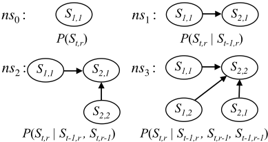
Multi-dimensional Markov chains (MdMCs) are an extension of higher-order Markov chains that relax the network structure even further, allowing any surrounding state in a multi-dimensional graph to be included. For example, the CPD defining the MdMC in Figure 2 (ns3) can be written as P(St↪r♣St-1↪r↪ St↪r-1↪ St-1↪r-1). Notice that there are other combinations of previous states that satisfy the definition of an order three MdMC. By redefining what a previous state can be in this way, the model is able to more easily capture relations from two-dimensional training data, as shown in our previous work [Snodgrass and Onta˜n´on, 2014]
Map Representation
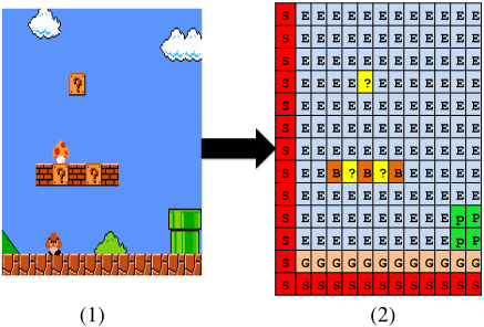
A map is represented by an h ⇥ w two-dimensional array, M, where h is the height of the map, and w is the width. Each cell of M is mapped to an element of S, the set of tile types which correspond to the states of the MdMC. Figure 1 shows a portion of a Super Mario Bros. map (left) and how that portion is represented as an array of tiles (right). Notice, we added sentinel tiles to the map to signify the boundaries.
Training
Training an MdMC requires two things: 1) the network structure and 2) training maps. Figure 2 shows example network structures that can be used to train an MdMC. Training happens in two steps: Absolute Counts and Probability Estimation. First, given the network structure, the number of times each tile follows each tile configuration is counted. Next, the probability distribution of the MdMC is estimated from these counts as the observed tile frequencies in the training data.
Sampling
A map is sampled with an MdMC one tile at time, starting, for example, in the bottom left corner, and completing an entire row before moving onto the next row. In more detail, a map is sampled in the following way: Given a desired map size, h ⇥ w, and a trained MdMC as described above, we probabilistically choose a tile based on the configuration of previous tiles and probability distribution of the trained chain.
While sampling, this method may encounter a set of previous tiles that was not seen during training. The probability estimation would thus have not been properly estimated (absolute counts would be 0). We call this an unseen state. We incorporate two strategies to avoid unseen states: look-ahead and fallback. These methods attempt to sample with the condition that no unseen states are reached. The look-ahead process samples a fixed number of tiles in advance, trying to ensure that no unseen state is reached. If the look-ahead is unsuccessful and a tile cannot be found that results in no unseen states, then our method falls back to an MdMC trained with a simpler network structure. In our experiments, we start with network structure ns3 (shown in Figure 2), which can fall back to ns2, which itself can fall back to ns1, and then to ns0, the raw distribution of tiles in the training maps. For more details on this training and sampling approach, the reader is referred to [Snodgrass and Onta˜n´on, 2014].
3 Constraining Sampling
The MdMC model explained above is able to sample new maps in the domain of the training data. However, the only way to affect the output maps is to modify the configuration of the MdMC or use different training maps, but these methods do not provide the user with intuitive control over the output maps, which is desirable [Togelius et al., 2013]. Furthermore, those methods of control do not give any guarantees that the desired traits will be present in the output maps.
To address the issue of controlling the output, we propose an approach where the user provides a set of constraints. Thus, we need methods for sampling maps that will uphold these constraints, which we describe below. We define two types of constraints:
- ÷ Simple Constraints: These constraints take a section of a map (or an entire map) as input, and return a cost representing the degree to which the provided section violates the constraint. The cost is 0 if the constraint is satisfied, and some positive value otherwise. Formally, c : M ! [0↪1), where c is the constraint function, and M is the section of the map.
- ÷ Location-Aware Constraints: These constraints take the entire map as input. They return a set of sections of the map that if resampled may allow the map to satisfy the constraint, as well as the total cost of c over M in the range of [0↪1), where 0 is satisfied and more positive costs are progressively less satisfied. Formally, c : M ! (2S ↪ [0↪1)), where c and M are as above, and 2S is the set of all subsets of map sections. We use c(m)▷cost and c(m)▷sections to represent the cost and sections returned by constraint c in map m. Notice, location-aware constraints could be used as simple constraints by ignoring the returned map sections.
An example of a simple constraint for Super Mario Bros. could be one that is satisfied if there is a path from the beginning to the end of the map, whereas a location-aware constraint could be one that is satisfied if each rows contains nonempty tiles, and otherwise returns the empty rows.
The set of constraints used in our experiments for each of our domains is described in Section 4.2. Next, we describe our algorithms for sampling a map that abides by the provided constraints using a multi-dimensional Markov chain. Notice that not all algorithms support both types of constraints. That is, an algorithm may require specific sections in the map to resample, whereas another algorithm may only require the cost associated with the constraint.
3.1 Generate and Test
The algorithm for this approach can be seen in Algorithm 1. This algorithm is the simplest; it follows a standard generate and test methodology. It takes a set of simple constraints, C, and the desired height and width of the output map, and starts by sampling a new map of the desired dimensions using the MdMC function (line 2), as described in Section 2.2. It then determines whether the map satisfies the provided constraints (line 3) by checking if the cost is 0 over all constraints. If it is not, the loop repeats, and an entirely new map is sampled.
3.2 Violation Location Resampling
This approach can be seen in Algorithm 2. At a high level, this algorithm works by sampling a new map and determining
Algorithm 1 GenerateAndTest(width ↪ height ↪ C)
1: repeat 2: Map =MdMC([0, 0], [width↪ height]) 3: until (Pc2C c(Map)) = 0 4: return MapAlgorithm 2 ViolationLocationResampling(w↪ h↪ C)
1: Map =MdMC([0, 0], [w↪ h]) 2: while (Pc2C c(Map)▷cost) > 0 do 3: for all c 2 C do 4: for all ([x1↪ y1]↪ [x2↪ y2]) 2 c(Map)▷sections do 5: for all ci 2 C do 6: costci = ci(Map[x1↪ y1][x2↪ y2])▷cost 7: end for 8: repeat 9: m = MdMC([x1↪ y1]↪ [x2↪ y2]) 10: for all ci 2 C ∩ c do 11: if costci > ci(m)▷cost then 12: GoTo line 9 13: end if 14: end for 15: until c(m)▷cost < costc 16: Map[x1↪ y1][x2↪ y2] =m 17: end for 18: end for 19: end while 20: return Mapwhich sections of the map should be resampled according to the constraints. Next, it resamples each of those sections until the cost of that section is reduced with regards to the current constraint (without raising the cost of any other constraints). Afterwards, if any constraints are not satisfied, the process of finding and resampling sections is repeated.
In more detail, this algorithm takes the dimensions of the output map and a set of location-aware constraints, C, and returns a map satisfying those constraints. The algorithm first samples a new map, Map (line 1). Next, if any constraints are unsatisfied (line 2), then for each constraint, c 2 C (line 3), it iterates over the sections which violate constraint c (line 4). It then records the cost of the current section according to each constraint (lines 5-7). When checking the cost of a section, we use the location-aware constraint as a simple constraint. The algorithm then samples a new section, m, of the same dimensions as the current section (line 9), and checks if the cost of m is greater than the previous cost for any other constraint (lines 10-14). If so, m is resampled, and cost checking is repeated. If the cost with regards to the other constraints is not raised, then m is only accepted if the cost with regards to the current constraint, c, is lowered (line 15). This process of finding violated sections and improving their costs is repeated until all constraints return cost 0 (line 2).
3.3 Incremental Sampling
This approach can be seen in Algorithm 3. This algorithm samples a map one section of the map at a time, resampling a section as needed until it satisfies the provided constraints.
Algorithm 3 IncrementalSampling(SecW ↪ h↪ n↪ C)
1: Map = empty map 2: for i = 0 !n-1 do 3: repeat 4: m =MdMC([i ⇥SecW, 0], [(i+1)⇥SecW↪ h]) 5: until (Pc2C c(m)) = 0 6: Map[i ⇥SecW, 0][(i+1)⇥SecW↪ h] =m 7: end for 8: return MapFor simplicity, we explain a version of the algorithm that assumes sections follow each other horizontally to the right. However, this ordering is domain dependent. Changing the ordering requires only modifying the indices passed to the MdMC function (line 4) and used during rewriting (line 6).
This algorithm takes the width of the sections to be sampled, SecW, the height of the map, h, the number of sections in a complete map, n, and a set of simple constraints, C. It first initializes an empty map, Map (line 1). Next, for each section to be sampled (line 2), it samples that section using the MdMC function and stores the newly sampled section in m (line 4). The algorithm then checks whether m satisfies the given constraints (i.e., the total cost of m over all constraints is 0, line 5). If m does not satisfy the constraints, it is resampled. Otherwise, m is appended to Map (line 6).
4 Experiments
We test our algorithms by sampling maps for two classic video games (Super Mario Bros. and Kid Icarus). 1 The remainder of this section describes these domains, and the specific constraints used in each domain, before elaborating on our experimental set-up and reporting the obtained results.
4.1 Domains
Super Mario Bros.: is a platforming game with linear maps (as defined by [Dahlskog et al., 2014]). The player traverses the maps from left to right while avoiding enemies and holes to complete the level. Our training set is 16 maps from Super Mario Bros. and Super Mario Bros.: The Lost Levels.
KidIcarus: is a platforming game with linear (albeit vertically oriented) maps. The player traverses the maps from bottom to top while avoiding hazards and holes to complete the level. Our training set includes 6 vertically-oriented maps from Kid Icarus.
4.2 Constraints
We defined constraints for each domain ranging from aesthetic constraints to playability constraints. Below we outline each constraint for each domain. Constraints listed with a with a ÷ are simple constraints, and those listed with a are location-aware constraints. Recall that location-aware constraints can be used as simple constraints, but simple constraints cannot be used as location-aware constraints.
1 All datasets used in our experiments can be downloaded from https://sites.google.com/site/sampsnodgrass
Each constraint that enforces an interval has two settings: an easy setting (denoted below by E) that is tuned to the average value over the training maps plus a standard deviation for the maximum value and minus a standard deviation for the minimum value, and a hard setting (denoted below by H) that sets the minimum value to the average and the maximum value to the average plus two standard deviations .
For Super Mario Bros. we used the following constraints:
- Number-of-Pipes(min↪max): To satisfy this constraint, a map must contain a number of pipes falling within [min↪max]. If not, sections where pipes can be added or removed are returned. E = Number-ofPipes(1↪ 13), H = Number-of-Pipes(7↪ 19).
- Number-of-Enemies(min↪max): To satisfy this constraint, a map must contain a number of enemies falling within [min↪max]. If not, sections where enemies can be added or removed are returned. E = Number-ofEnemies(11↪ 31), H = Number-of-Enemies(21↪ 41).
- Number-of-Gaps(min↪max): To satisfy this constraint, a map must contain a number of gaps falling within [min↪max]. If not, sections where gaps can be added or removed are returned. E = Number-ofGaps(4↪ 12), H = Number-of-Gaps(8↪ 16).
- Longest-Gap(min↪max): To satisfy this constraint, the longest gap's length must fall within [min↪max]. If not, sections where gaps can be modified are returned. E = Longest-Gap(4↪ 8), H = Longest-Gap(6↪ 10)
- No-Ill-Formed-Pipes(): To satisfy this constraint, a map must contain no ill-formed pipes. An ill-formed pipe is any pipe not consisting of both left and right pipe tiles or without solid tiles beneath it (pipes that extend to the bottom of the map are not considered ill-formed). Sections containing ill-formed pipes are returned.
- Playability(): To satisfy this constraint, a path must exist from the beginning to the end of the map. This is tested with Summerville's A* agent [Summerville et al., 2015]. Unplayable sections are returned for resampling.
- ÷ Linearity(min↪max): To satisfy this constraint, the linearity of the map must fall within [min↪ max ]. Linearity is the sum of distances from a best-fit line, where solid tiles are treated as points [Smith and Whitehead, 2010]. E = Linearity(280↪ 566), H = Linearity(423↪ 709)
- ÷ Leniency(min↪max): To satisfy this constraint, the leniency of the map must fall within [min↪max]. Leniency is the weighted sum of the number of enemies and gaps weighted by length [Smith and Whitehead, 2010]. E = Leniency(14↪ 46), H = Leniency(30↪ 62)
Notice, linearity and leniency are used as global constraints, and as such are only checked on an entire map, not sections. For Kid Icarus we used the following constraints:
- Number-of-Hazards(min↪max): To satisfy this constraint, a map must contain a number of hazards falling within [min↪max]. If not, sections where hazards can be added or removed are returned. E = Number-ofHazards(0↪ 27), H = Number-of-Hazards(13↪ 41)
- Longest-Gap(min↪max): To satisfy this constraint, the longest gap's length must fall within [min↪max]. If not, sections where gaps can be modified are returned. E = Longest-Gap(10↪ 12), H = Longest-Gap(11↪ 13)
- Average-Platform-Length(min↪max): To satisfy this constraint, the average length of the platforms in a map must fall within [min↪max]. If not, sections where platforms can be modified are returned. E = Average-Platform-Length(3↪ 4), H = AveragePlatform-Length(3▷5↪ 4▷5)
- Playability(): To satisfy this constraint, a path must exist from the beginning to the end of the map. This is tested by checking the distances between platforms. Unplayable sections are returned for resampling.
The section sizes used are explained in the following section.
4.3 Experimental Setup
We tested our algorithms by training MdMCs (as described in Section 2.2) on the training maps. The employed MdMC approach allows configuring parameters to better suit certain domains (see [Snodgrass and Onta˜n´on, 2014]). In our experiments we set those parameters to the following values: for Super Mario Bros. we configure an MdMC with rowsplits = 12 and look-ahead = 3. For Kid Icarus we configure an MdMC with rowsplits = 10 and look-ahead = 3, which were the most promising configurations over some preliminary runs without constraints . We use these MdMCs to sample new maps within our constraint enforcement algorithms. However, not all algorithms support all the constraints we defined. Thus, we experimented with three subsets of constraints:
- ÷ IS: For Super Mario Bros., IS =¶Playability, No-illFormed-Pipes♦. For Kid Icarus, IS =¶Playability♦. These sets pair with all three of our algorithms.
- ÷ VLR: For Super Mario Bros., VLR = IS [ ¶Number-of-Pipes, Number-of-Enemies, Number-ofGaps, Longest-Gap♦. For Kid Icarus, VLR = IS [ ¶Number-of-Hazards, Longest-Gap, Average-PlatformLength♦. These sets pair with the Violation Location Resampling and Generate and Test algorithms.
- ÷ GT : For Super Mario Bros., GT = VLR [ ¶Linearity, Leniency♦. For Kid Icarus GT = VLR. These sets pair with the Generate and Test algorithm.
We will use the subindex e to represent easy constraint value settings and h to represent hard constraint value settings.
Location-aware constraints experiments return sections of size 10⇥12 for Super Mario Bros. and 16⇥10 for Kid Icarus (width by height). The constraints select the sections to return via a sliding window approach. Each of the windows tested where a violation was found is returned by the constraints; overlapping windows are combined.
For the Incremental Sampling algorithm we used the same section sizes as above. With these section sizes, Super Mario Bros. maps are one section tall, and Kid Icarus maps are one section wide. We sampled maps that are 21 sections long for Super Mario Bros. and 17 section tall for Kid Icarus, as these are typical sizes observed in the training sets.
During preliminary experiments we found that occasionally an algorithm would get stuck and be unable to satisfy the constraints (or take an excessive amount of time to do so). Thus, in our experiments, we limit the number of times a map could be resampled. That is, given a map of L sections, we limit the number of total sections sampled to 50L, after which we consider the execution to have failed. Note that on a standard laptop the baseline MdMC approach is able to sample 50 complete maps in about one second.
In our preliminary experiments, we tested our sampling algorithms with a uniform distribution MdMC to determine whether the algorithms were overwriting the distribution by enforcing the constraints. We found that none of the algorithms paired with the uniform distribution MdMC could satisfy even the simplest constraints, showing the trained MdMC probability distribution is an important part of sampling.
To evaluate our algorithms, we sampled 100 maps with each viable combination of algorithm and set of constraints. We recorded the percentage of maps sampled that satisfied the provided constraints (Satisfied) and the average number of sections sampled per satisfied map (Attempts). Note, Attempts includes the initial sections sampled as well as the sections resampled. Lastly, we compare our algorithms against a baseline, where we sampled 100 maps using an MdMC with the same configuration as our algorithms, but without enforcing any constraints. We then compute how many of those maps satisfy the various sets of constraints.
4.4 Results
Table 1 shows the results of our experiments. Rows labeled with "MdMC" are the baseline model, as in Section 2.2 (without considering any constraints), where the number of maps satisfying each set of constraints is computed afterwards.
As expected, all of our algorithms (excluding the Generate and Test algorithm when used with Kid Icarus) were able to produce a higher percentage of maps satisfying the provided constraints than the MdMC alone was able to. This suggests that by providing constraints, we are able to guide the sampler towards more desirable maps.
An interesting trend, when looking at the Super Mario Bros. results, is that when comparing our three algorithms using the VLRe↪VLRh, and IS constraints the three algorithms achieve the same satisfaction percentage for each set of constraints, but the Violation Location Resampling (VLR) and the Incremental Sampling (IS) algorithms outperform the Generate and Test (G+T) algorithm with respect to the number of sections sampled. This is because G+T must resample all sections if a constraint is violated anywhere, whereas VLR and IS selectively resample particular sections in violation of the constraints. However, in Kid Icarus, notice that VLR outperforms IS in terms of sections sampled (VLR, sampling fewer than half as many sections as IS). This may stem from the dependence a section has on the previous section in Super Mario Bros., where each row continues from the row of the previous section, whereas in Kid Icarus a section is far less dependent on the previous section, due to the vertical orientation of the map, which can lead to more diversity in the sections being sampled, and therefore may require more resamplings to produce a satisfactory section.

Furthermore, in Kid Icarus, the VLR and IS algorithms both outperform the G+T algorithm, achieving the same percentage of satisfied maps, where the G+T algorithm and the baseline were unable to produce any. This is a remarkable result as it indicates that with the proper constraints, an MdMC can sample usable maps for domains which are beyond the reach of current statistical sampling-based PCG methods.
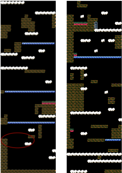
Figure 3 shows a portion of a map sampled using the VLR algorithm enforcing the VLRh constraints, as evidenced by the drastically varying heights and large number of enemies. Figure 4 (left) shows a portion of an unsatisfied map sampled using the G+T algorithm enforcing the GT e constraints, where a gap that is too long to jump over is circled. Figure 4 (right) shows a portion of a map sampled using the VLR algorithm enforcing the VLRe constraints.
| Super Mario Bros. | KidIcarus | ||||
|---|---|---|---|---|---|
| Alg. | C | Satisfied | Attempts | Satisfied | Attempts |
| MdMC | GTe | 42% | 21▷00 | 0% | NA |
| MdMC | GTh | 1% | 21▷00 | 0% | NA |
| MdMC | VLRe | 50% | 21▷00 | 0% | NA |
| MdMC | VLRh | 3% | 21▷00 | 0% | NA |
| MdMC | IS | 72% | 21▷00 | 0% | NA |
| G+T | GTe | 100% | 75▷18 | 0% | NA |
| G+T | GTh | 59% | 419▷29 | 0% | NA |
| G+T | VLRe | 100% | 72▷66 | 0% | NA |
| G+T | VLRh | 75% | 435▷96 | 0% | NA |
| G+T | IS | 100% | 54▷81 | 0% | NA |
| VLR | VLRe | 100% | 23▷01 | 94% | 275▷04 |
| VLR | VLRh | 75% | 176▷43 | 0% | NA |
| VLR | IS | 100% | 21▷32 | 100% | 98▷36 |
| IS | IS | 100% | 21▷02 | 100% | 210▷76 |
5 Conclusions
This paper presented three algorithms for enforcing constraints while sampling using multi-dimensional Markov chains (MdMCs), tested in the domain of video game map generation. We found our algorithms provide the user with more control over the qualities of the output maps than sampling with the MdMC alone, though the Violation Location Resampling and Incremental Sampling algorithms converge to a solution more quickly than the Generate and Test algorithm. Additionally, the algorithms produced playable maps for Kid Icarus which we were unable to do previously with the standard MdMC approach, suggesting these algorithms will enable us to sample maps for domains which are beyond the reach of current statistical sampling-based PCG methods. Moreover, while the proposed algorithms were evaluated in the context of video game map generation, they constitute a general approach to constrained sampling of Markov models, which may have applications beyond video games (e.g., music generation, texture synthesis, and text generation).
For our future work, we would like to explore sampling algorithms that can handle a wider range of constraints. Additionally, we would like to evaluate our methods in more complex video games, such as puzzle-platformers (e.g., Loderunner), where complex paths through the maps are important.
@inproceedings{ijcai2016p116,
  title     = {Controllable Procedural Content Generation via Constrained Multi-Dimensional Markov Chain Sampling},
  author    = {Snodgrass, Sam and Ontañón, Santiago},
  booktitle = {Proceedings of the Twenty-Fifth International Joint Conference on
               Artificial Intelligence, {IJCAI-16}},
  publisher = {AAAI Press / International Joint Conferences on Artificial Intelligence},
  editor    = {Subbarao Kambhampati},
  pages     = {780--785},
  year      = {2016},
  month     = {7},
  url       = {https://ijcai.org/proceedings/2016/116},
}
TY - CPAPER TI - Controllable Procedural Content Generation via Constrained Multi-Dimensional Markov Chain Sampling AU - Snodgrass, Sam AU - Ontañón, Santiago T2 - Proceedings of the Twenty-Fifth International Joint Conference on Artificial Intelligence, IJCAI-16 PB - AAAI Press / International Joint Conferences on Artificial Intelligence PY - 2016 SP - 780 EP - 785 UR - https://ijcai.org/proceedings/2016/116 ER -Copied
Machine-readable versions of this paper, for tools and AI agents:





