
Interactive Martingale Boosting
Proceedings of the Twenty-Fifth International Joint Conference on Artificial Intelligence. Pages 841-846.
Abstract
We present an approach and a system that explores the application of interactive machine learning to a branching program-based boosting algorithm- Martingale Boosting. Typically, its performance is based on the ability of a learner to meet a fixed objective and does not account for preferences (e.g. low false positives) arising from an underlying classification problem. We use user preferences gathered on holdout data to guide the two-sided advantages of individual weak learners and tune them to meet these preferences. Extensive experiments show that while arbitrary preferences might be difficult to meet for a single classifier, a non-linear ensemble of classifiers as the one constructed by martingale boosting, performs better.
- [Alpaydin and Kaynak, 1998] Ethem Alpaydin and Cenk Kaynak. Cascading classifiers. Kybernetika, pages 369- 374, 1998.
- [Fan et al., 1999] Wei Fan, Salvatore J Stolfo, Junxin Zhang, and Philip K Chan. Adacost: misclassification cost- sensitive boosting. In ICML, volume 99, pages 97-105.
- [Fletcher, 2013] Roger Fletcher. Practical methods of opti- mization. John Wiley & Sons, 2013.
- [Foo et al., 2007] Chuan-sheng Foo, Chuong B Do, and An- drew Ng. Efficient multiple hyperparameter learning for log-linear models. In Advances in neural information pro- cessing systems, pages 377-384, 2007.
- [Freund and Schapire, 1997] Yoav Freund and Robert E. Schapire. A decision-theoretic generalization of on-line learning and an application to boosting. Journal of Com- puter and System Sciences, pages 119-139, 1997.
- [Freund, 1995] Yoav Freund. Boosting a weak learning al- gorithm by majority. Inf. Comput., pages 256-285, 1995.
- [Gavrilut et al., 2009] Dragos Gavrilut, Mihai Cimpoesu, Dan Anton, and Liviu Ciortuz. Malware detection us- ing machine learning. In International Multiconference on Computer Science and Information Technology, pages 735-741. IEEE, 2009.
- [Kapoor et al., 2010] Ashish Kapoor, Bongshin Lee, Desney Tan, and Eric Horvitz. Interactive optimization for steer- ing machine classification. In Proceedings of the SIGCHI Conference on Human Factors in Computing Systems, pages 1343-1352, New York, NY, USA, 2010. ACM.
- [Kapoor et al., 2012] Ashish Kapoor, Bongshin Lee, Desney S Tan, and Eric Horvitz. Performance and preferences: Interactive refinement of machine learning procedures. In AAAI, 2012.
- [Kaynak and Alpaydin, 2000] Cenk Kaynak and Ethem Al- paydin. Multistage cascading of multiple classifiers: One man's noise is another man's data. In Proceedings of the Seventeenth International Conference on Machine Learn- ing, pages 455-462, San Francisco, CA, USA, 2000.
- [Kearns and Mansour, 1996] Michael Kearns and Yishay Mansour. On the boosting ability of top-down decision tree learning algorithms. In Proceedings of the Twenty- eighth Annual ACM Symposium on Theory of Computing, pages 459-468, New York, NY, USA, 1996. ACM.
- [Kearns and Valiant, 1994] Michael Kearns and Leslie Valiant. Cryptographic limitations on learning boolean formulae and finite automata. Journal of the ACM, pages 67-95, 1994.
- [Long and Servedio, 2005] Philip M. Long and Rocco A. Servedio. Martingale boosting. In Proceedings of the 18th Annual Conference on Learning Theory, pages 79- 94, Berlin, Heidelberg, 2005. Springer-Verlag.
- [Long and Servedio, 2008] Phil Long and Rocco Servedio. Adaptive martingale boosting. In Advances in Neural In- formation Processing Systems, pages 977-984, 2008.
- [Mansour and McAllester, 2002] Yishay Mansour and David McAllester. Boosting using branching programs. Journal of Computer and System Sciences, 64:103-112, 2002.
- [Masnadi-Shirazi and Vasconcelos, 2011] Hamed Masnadi- Shirazi and Nuno Vasconcelos. Cost-sensitive boosting. Pattern Analysis and Machine Intelligence, IEEE Trans- actions on, 33(2):294-309, 2011.
- [Mosteller and Tukey, 1968] Frederick Mosteller and John W Tukey. Data analysis, including statistics. 1968.
- [Olshen and Stone, 1984] L Breiman JH Friedman RA Ol- shen and Charles J Stone. Classification and regression trees. Wadsworth International Group, 1984.
- [Schapire, 1990] Robert E. Schapire. The strength of weak learnability. Machine Learning, pages 197-227, 1990.
- [Stone, 1974] M. Stone. Cross-Validatory Choice and As- sessment of Statistical Predictions. Journal of the Royal Statistical Society, (2):111-147, 1974.
- [Viola and Jones, 2001] Paul Viola and Michael Jones. Rapid object detection using a boosted cascade of simple features. In Proceedings of the 2001 IEEE Computer So- ciety Conference on Computer Vision and Pattern Recog- nition, pages I-511. IEEE, 2001.
- [Wu et al., 2008] Shan-Hung Wu, Keng-Pei Lin, Chung-Min Chen, and Ming-Syan Chen. Asymmetric support vector machines: low false-positive learning under the user toler- ance. In Proceedings of the 14th ACM SIGKDD interna- tional conference on Knowledge discovery and data min- ing, pages 749-757, New York, NY, USA, 2008. ACM.
- [Yih et al., 2006] Wen-tau Yih, Joshua Goodman, and Geoff Hulten. Learning at low false positive rates. In CEAS, 2006.
References were extracted automatically from the PDF and may contain errors.
Full text extracted automatically from the PDF; figures, tables and equations may differ. The PDF is the version of record.
1 Introduction
Boosting algorithms are efficient procedures that, given access to a weak learning algorithm, use weak learners to construct a strong learner with arbitrarily low error on any given probability distribution. Kearns and Valiant [Kearns and Valiant, 1994] defined a weak learning algorithm as the one that produces a hypothesis that performs slightly better than random on that distribution. There is a large body of work [Schapire, 1990; Freund, 1995; Kearns and Mansour, 1996] that has proposed and studied several boosting algorithms for their theoretical soundness. However, Martingale boosting (MB) [Long and Servedio, 2005], with its proven tolerance to noise and well-defined structure, might be a promising approach to practical classification problems. The algorithm assumes access to a weak learning algorithm with a two-sided (on positive and negative class) advantage γ, such that the accuracy of each weak learner is at least 12 +γ. However, a practical application might prefer differential two-sided advantages (as we discuss next) and these are not explicitly modeled.
Depending on the choice of the learning algorithm, a learner usually seeks a hypothesis that meets a fixed objective, such as "minimize logistic loss" or "maximize classification accuracy". Such a predefined objective might fail to capture the preferences that are inherent in the underlying classification problem. For instance, in case of spam classification [Yih et al., 2006], classification of a non-spam document as spam might incur a higher utility cost, than a spam document which is undetected. On the other hand, in the medical domain, false negatives are indicative of missed diagnosis and having them might be catastrophic.
In general, rather than seeking a hypothesis to meet a predefined preference, a learner might benefit from a human-inthe-loop approach where such preferences are specified by users in an interactive "dialog" with the model. These preferences in turn guide the two-sided advantages of the individual weak learners.
2 RelatedWork
Classification with asymmetric costs: There is a body of research that explores the thesis that different learners might make errors on different training examples and therefore proposes a multistage cascade [Gavrilut et al., 2009; Kaynak and Alpaydin, 2000] of classifiers. The classification of an example is either a collective decision of all the classifiers in the cascade [Gavrilut et al., 2009] or a classifier might only receive examples that are rejected by the previous classifiers [Kaynak and Alpaydin, 2000; Viola and Jones, 2001; Alpaydin and Kaynak, 1998]. Training using utility has also been explored by [Wu et al., 2008], where, they propose an Asymmetric Support Vector Machine (ASVM) that accounts for tolerance to false-positives in its objective. Another approach known as stratification [Olshen and Stone, 1984] works by re-weighting instances, and is explored by [Yih et al., 2006] for the problem of spam classification. Cost-sensitive boosting-based approaches [Fan et al., 1999; Masnadi-Shirazi and Vasconcelos, 2011] also incorporate cost in instance reweighting, however, they (1) assume prior knowledge of misclassification cost (2) weight training instances while we weight holdout data.
Boosting: Boosting methods work by constructing several weak classifiers that collectively give rise to a strong classifier. While AdaBoost [Freund and Schapire, 1997] takes a linear combination of these classifiers, [Freund, 1995] uses the majority vote to label instances. One of the drawbacks of these algorithms is their intolerance to noisy data and this has led to a growing interest in non-linear branching programsbased boosting approaches. Kearns et al. explored the boosting ability of top-down decision tree algorithms but identified the exponential growth of tree size as a problem. Branching programs are a generalization of decision trees and can represent functions that are significantly more powerful [Mansour and McAllester, 2002]. Recently [Long and Servedio, 2005] proposed an approach called martingale boosting that constructs branching programs with well-defined structure and has an elegant graph walk-based analysis. Adaptive martingale boosting [Long and Servedio, 2008] retains the noise tolerance of the previous algorithm while taking advantage of varying strengths of the weak learners in achieving a stronger bound on the overall error.
Interactive machine learning: Instead of focusing on one particular target, [Kapoor et al., 2012] enable users to explore and express preferences about the operation of classification models. The underlying computational procedure then tunes the model hyper-parameters accordingly. However, their approach might fail to meet an arbitrary user input.
3 Our Contributions
We present an approach and a system called interactive martingale boosting (IMB) to interactively tune the performance of a classifier. We show how ideas from interactive machine learning could be applied to martingale boosting, not only in specifying user preferences, but also in tuning the individual advantages of the weak learners of MB. While our approach is based on martingale boosting, unlike them, we do not assume a predefined target. We introduce separate two-sided advantages on the positive and negative instances and tune them separately, while guided by the user specified preferences. Additionally, we are perhaps the first ones to perform extensive experiments with multiple datasets to demonstrate the feasibility and performance of MB, adaptive MB, and our interactive MB approach. We show, through experiments 1 , that in comparison to the single level interaction of [Kapoor et al., 2012], our approach, with its multiple levels of interaction, allows a user to browse through several additional models in the hypothesis space, thereby doing better in meeting user preferences. Our tooling systematically guides users in their interactive dialog with the model learner by tracking the trajectory of the model performance.
4 Approach
We start by formally defining the problem, describing our interactive martingale boosting approach followed by a description of tuning of its individual weak learners.
1 Code available at https://github.com/kulashish/adaptivemb
4.1 ProblemDefinition
Let X be the set of input examples sampled from a distribution D and ¶0↪ 1♦ be the output labels. We are required to learn (on subset XTrain ⇢ X) a target function c : X ! ¶0↪ 1♦, where, c best satisfies a user defined accuracy criterion. Based on the underlying usecase, users might prefer a differential misclassification cost. Typically, deciding an acceptable misclassification cost requires iterative tuning of the classifier on a holdout (or tuning) set XTune.
Definition 1. Let D+ denote the distribution D restricted to the positive examples ¶x 2 X : c(x) = 1♦ and let D- denote D restricted to the negative examples ¶x 2 X : c(x) = 0♦. A hypothesis h : X ! ¶0↪ 1♦ is said to have two-sided advantages γ+ and γ- with respect to D+ and D-, respectively, if it satisfies Prx2D+[h(x) = 1] ≥ 12 + γ+ and Prx2D-[h(x) = 0] ≥ 12 + γ-.
Here, 12 + γ+ and 12 + γ- are the desired accuracies Acc+des = TP◁(TP +FN) and Acc-des = TN◁(TN +FP ) on D+ and D- respectively. How do we enable a user to decide an acceptable classifier performance γ+ and γ-? How do we tune a classifier to best meet these user preferences? These are the research challenges that we address through our interactive approach.
4.2 User Interaction through ConfusionMatrix
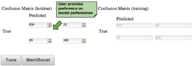
Users specify the classifier preferences through an interactive visualization that displays the confusion matrix on a holdout dataset (Refer to Figure 1). This is inspired from the observation of [Kapoor et al., 2010] that an interactive confusion matrix enables users to more effectively estimate misclassification risks. Users specify their desire by editing the number of instances classified in each cell. For instance, users could specify their model preference by reducing the number of false positives on the holdout set from 70 to 65. This translates into a user preference on the desired accuracy Acc-des and effectively on the advantage γ- = Acc-des - 12 . The underlying procedure then tunes the model hyperparameters in an attempt to return a model that best meets this preference. If a feasible solution is obtained, the holdout confusion matrix is updated and this often affects the values in other cells. Otherwise, a notification of inability to meet the preferences is provided to the user. The user continues this interactive model exploration until a satisfactory model is obtained.
4.3 Interactive Martingale Boosting
User preferences, γ+ or γ-, on a model's performance are used to tune the classification model in an attempt to meet these preferences. [Kapoor et al., 2012] presented an efficient numerical procedure that tunes the hyperparameters of a model in response to preferences specified through an interactive confusion matrix. Often, a single model fails to satisfy arbitrary user specifications (Refer to section 5.4). We propose an approach called Interactive Martingale Boosting (IMB) based on a non-linear ensemble of interactive classifiers. Choice of martingale boosting [Long and Servedio, 2005] is motivated from its simple non-linear structure and its tolerance to noise, which is often important for practical applications.
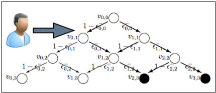
Let ML be a L-stage martingale boosting program resulting in a L + 1 layered directed acyclic graph (DAG). Each node in the DAG is labeled as vi↪j, where j is the index of a layer, j 2 ¶0↪ 1↪ ▷ ▷ ▷ ↪L♦ and for a node at layer t, i 2 ¶0↪ 1↪ ▷ ▷ ▷ ↪ t♦. v0↪0 is the root node. The root node receives all the training XTrain and holdout XTune instances, which are used to grow a MB program as described next. Let D+ i↪j and Di↪j be the distributions of positive and negative examples reaching node vi↪j. At every node, we train a classification model hi↪j and evaluate it on the holdout set at that node to generate a local confusion matrix Ci↪j . Each node vi↪j has two outgoing edges labeled 0 and 1, that connect to nodes vi↪j+1 and vi+1↪j+1, respectively (Figure 2 shows a 3-stage MB). Each training and holdout instance is routed along the edge labeled hi↪j(x) until it reaches a leaf node vl↪L where its final label is set to 0 if l L◁2 and is set to 1 otherwise. The final label of an instance thus depends on its classification by the individual classifiers on its way from the root node to the leaf. These final labels give rise to a global confusion matrix CL for the L-stage MB program. Users interact with the cells in this confusion matrix, thereby specifying the desired advantages γ+ and γ- for the MB classifier. These global specifications are used to derive local specifications γ+ i↪j and γi↪j at node vi↪j and each model hi↪j is tuned accordingly.
Granularity of Interaction
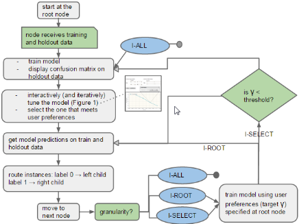
The choice of node-level advantages γ+ i↪j and γi↪j depends on the granularity of user interaction. For relatively smaller MB programs, a user can interactively tune the classifier at every node (we refer to this as I-ALL) and view its impact on the overall performance of the boosted classifier. However, this human effort is quadratic in the number of levels in a MB program and might become unfeasible even for a moderate number of levels. In such cases, user preferences might be gathered only on the global confusion matrix CL (we refer to this as I-ROOT). The resultant γ+ and γ- could then be used as targets in automatically tuning the node-level classifiers. Alternatively, the distinct advantages of these individual learners, could be used to identify particularly "weak" nodes. Following the spirit of active learning, a user could then be prompted to interactively tune only these learners, in an attempt to learn a boosted classifier that meets user preferences. We refer to this as I-SELECT and it attempts to achieve a middle ground between I-ROOT and I-ALL. We study the effect of some of these granular interactions in the evaluation section. Figure 3 shows the system flow for each of these levels of granular interactions.
Early Node Freezing
As the MB program grows top-down, the distribution of examples reaching at some of the nodes tends to be heavily biased towards a class label. This might typically happen at nodes at the extreme ends of a level, that usually have a better advantage for one class over others. These nodes could be "frozen" by labeling the instances reaching there with the label of the majority class, with little impact on the overall error rate. Similar to the approach used by Sampling MartiBoost [Long and Servedio, 2005], we freeze a node vi↪j if the minimum of the probabilities of a positive or negative instance reaching that node minb2¶+↪-♦ pbi↪j < ✏ L(L+1) for some error rate ✏.
Error Rate
The misclassification error on negative examples (FP-rate) ✏-i↪j at a node vi↪j is 12 - γi↪j . Based on the definition of the martingale program above, it is easy to see that the misclassification error ✏-(ML) of ML on negative examples is the fraction of negative examples reaching leaf nodes vl↪L where l 2 ¶L◁2+1↪ ▷ ▷ ▷ ↪ L♦. For L = 1, ✏-(M1) = ✏-0↪0 = 12 -γ0↪0 . Figure 2 shows a martingale program for L = 3, where the edges are labeled with the fraction of negative examples moving from a node at the tail of an edge, to the node at its head. It follows that the fraction of negative examples that make it to nodes v2↪3 and v3↪3 is given by
The error rate has a corresponding definition in terms of weights of paths in a directed acyclic graph for ML2 .
4.4 Node-level Model Tuning
The node-level model preferences γ+ i↪j and γi↪j are used to tune the hyperparameters of the classifier hi↪j. Often, grid search is employed to get a sub-optimal estimate of the hyperparameters such that it minimizes the holdout loss. Model selection using a holdout dataset is a standard technique used to avoid over-fitting the training data [Mosteller and Tukey, 1968; Stone, 1974]. While this approach works for a single hyperparameter, more sophisticated strategies are required for tuning multiple hyperparameters. We borrow the hyperparameter tuning approach from the work by [Kapoor et al., 2012] and describe it briefly here.
2 Refer to the supplement https://goo.gl/nWrioq
Consider a training set XTrain with corresponding labels drawn from Y 2 ¶1↪ ▷ ▷ ▷ ↪ k♦, let w be the model parameters and d represent the set of hyperparameters for our model. We wish to determine an updated model d⇤ in response to user preferences on a holdout confusion matrix. For the current model choice, we train the model on XT rain to obtain weights w⇤ and evaluate it on a holdout set XTune giving for each point x(i) 2 XTune, a k-dimensional vector y(i) = [y(i) c ]kc=1 , where y(i) c denotes the classification score for class c. A softmax transformation of y(i) results in a k-dimensional current state vector p(i) (d; w⇤ ), corresponding to the input point x(i) and model d. User preferences essentially express the desire to classify a point (1) as class b, encoded as a target state vector s(i) with all zeros except the bth component set to 1; (2) not as class b, in which case s(i) has bth component set to 0 and all other components set to 1◁(k-1); (3) with no change and thus s(i) = p(i) (d;w⇤ ). The goal is to minimize the difference between the target and current states and they use KL divergence as the objective function:
We use gradient descent with BFGS update [Fletcher, 2013] to solve the optimization problem. Note that we do not have to completely minimize the objective, but only minimize it up to a point that satisfies user specifications.
4.5 Gradient Computation
We use multinomial logistic regression as the node-level learner in our interactive martingale boosting approach. Multinomial LR is a simple and fast algorithm with low variance and a probabilistic output score. This makes it possible to systematically use predictions from individual weak learners in our larger boosted model and also allows us to extend to multiclass setting. Multinomial LR models the conditional probability P(y♣x;w) = exp(wT F(x↪ y))◁Z(x), where, F(x↪ y) is a vector valued mapping of (x↪ y) to a feature space and Z(x) = Py02Y exp(wT F(x↪ y0 )).
The parameters w are usually learned using regularized logloss minimization [Foo et al., 2007]:
where 12 wT Cw is the regularization term and C is the inverse covariance matrix of a Gaussian prior on the parameters w. Consider a setting, say, spam classification, where different subsets of parameter components (corresponding to single word features, bigram features etc.), might be constrained by different hyperparameters. Thus, C is usually parameterized by a hyperparameter vector d as the diagonal matrix C(d) = diag(exp(d)).
The hyperparameters are trained on the holdout data by solving the optimization:
subject to
Using the chain rule of differentiation, we get
where JTd is the Jacobian matrix comprising partial derivative of w⇤ with respect to d as defined by equation (6) in [Foo et al., 2007] and rwg(d;w⇤ ) is obtained by evaluating the gradient of equation (1) at w⇤ .
4.6 Multiclass Interactive Martingale Boosting
Martingale boosting naturally extends to the problem of multiclass classification under the strict assumption of k-sided advantage (Refer to the supplement).
5 Evaluation
We evaluate the effectiveness of interactive martingale boosting by performing experiments for the problem of binary classification on several UCI datasets including Spambase, Sonar, Ionosphere, and Liver, and for multiclass classification on Splice and Iris datasets. While some of these datasets are the same as those used by [Kapoor et al., 2012], others were chosen due to the applicability of this approach to medical and spam domains.
5.1 Interactive Tuning versus Grid Search
We assumed a separate regularization penalty per model parameter in equation (2) and tuned them using the interactive procedure. We validate the effectiveness of this procedure by comparing it with grid search on the Liver dataset. We performed an exhaustive search in the range 0 to 300 with a step size of 30, choosing hyperparameters for which the validation accuracy was the maximum. Grid search achieved an overall accuracy of 68▷84% on the test set versus 77▷06% achieved by the interactive refinement. This observation is consistent with that of Kapoor et al.
5.2 Effect of Base Learner and Boosting
We used multinomial LR and martingale boosting as our base learner and boosting algorithms respectively. What would be the effect of using a different base learner or boosting approach? We compare multinomial LR against RBF kernelbased classifier (choice of Kapoor et al.) and also evaluate the performance of AdaBoost (50 iterations) and MB (15 levels) on these base learners. Table 1 reports the average test accuracy across five splits (60% train and 40% test) of the dataset. Multinomial LR vs. RBF: Both the base classifiers show a comparable performance with LR performing slightly worse on Ionosphere and slightly better on Sonar. Base classifiers with interactive tuning: Interactive tuning does improve model accuracy with LR-Tune doing better than RBFTune. Models were tuned using 3-fold cross-validation within each train split and the best model was chosen. Base classifiers with boosting: Both AdaBoost and MB have an improved accuracy over that of base classifiers. As expected, MB, with its non-linear branching program-based structure, performed better than AdaBoost. While the choice of base classifier might slightly affect the model performance, both interactive tuning and MB, consistently improved the model performance.
| Dataset | RBF | LR | RBF- Tune* | LR- Tune | Ada- RBF | Ada- LR | MB- RBF | MB- LR |
|---|---|---|---|---|---|---|---|---|
| Ionosphere | 91.03 | 90.71 | 92.55 | 93.43 | 92.96 | 94.97 | 95.58 | 96.42 |
| Sonar | 85.67 | 86.75 | 86.9 | 91.02 | 87.72 | 89.87 | 90.38 | 91.08 |
5.3 How Effective is Interactive Martingale Boosting?
We tested the effectiveness of our procedure in a two-class classification task on the UCI Spambase dataset, with an aim of reducing false positives. We compare multinomial LR (LR), LR tuned using our interactive procedure (LR-Tune), martingale boosting (MB), martingale boosting with interactively tuned weak learner (MB-Tune) and finally, MB-Tune with early freezing of non-leaf nodes (MB-Tune-Freeze).
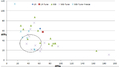
Figure 4 shows a scatter plot of FP-FN obtained by these procedures. The multiple data points for the martingale boosting-based approaches correspond to different number of levels of the branching program. The models were tuned to minimize the number of FPs as much as possible, and thus, the models in the lower half of the plot are more desirable and the ones in the lower left quadrant achieve a better overall accuracy. LR-Tune does marginally better than LR in achieving a lower number of FPs, but the interactive martingale boosting based approaches perform much better, both in reducing the number of false positives and in maximizing the overall accuracy.
5.4 Comparison with Other Methods
We compared the effectiveness of our approach with that of other approaches on UCI datasets. We report class-wise accuracy 3 and the overall accuracy obtained on the test set averaged over five splits (Refer to Table 2). Multinomial LR was used as the base classifier and the number of levels, L, of MB was empirically set to 15. Granularity of interaction was set to I-ROOT. Although the system allows for arbitrary user preferences, for ease of evaluation we tune all models in favor of one of the classes (as specified in the table), as is typical of applications in the spam (zero FPs) and medical (zero FNs) domains. We compare our approaches, MB-Tune(I-ROOT) and MB-Tune-Freeze (early node freezing) with multinomial LR (LR), LR with interactive tuning (LR-Tune), LR with AdaBoost (Ada), tuned LR with AdaBoost (Ada-Tune), adaptive MB (AMB), and adaptive MB with tuning (AMB-Tune).
3 Accuracy for a class = TP/(TP+FN)
Consistent with our earlier observation, effectiveness of the martingale boosting approach is apparent here as well. Further, interactively tuned MB, MB-Tune(I-ROOT), outperforms other approaches on all datasets. Accuracy on the favored class is generally higher than that achieved by MB and might come at the cost of reduced accuracy on the nonfavored class (as can be seen for Spambase). In other cases, accuracy on the non-favored class also improved and this could be attributed to a different routing of instances in the tuned MB. With early freezing of nodes, the results are only slightly worse, but with the advantage of a significant reduction in the number of nodes in the DAG. On the Spambase dataset for instance, 70 of the total 120 nodes got frozen. In adaptive MB, a node has more than two child nodes and an instance, based on its classification score, gets routed to an appropriate child node. Although adaptive MB has a better error bound in theory, in our observation, it seemed to over fit the training data. Its accuracy on the test data, even with tuning at the root node (AMB-Tune), is at times slightly worse than that of MB.
Comparison with Yih et al.: We evaluated the approach of [Yih et al., 2006] on the Sonar and Ionosphere datasets. However, it was not clear how to translate user preferences to the input that they expected. The best results we obtained among various inputs were Acc+: 79▷62%, Acc-: 94▷18%, Acc: 88▷57% on Ionosphere and Acc+: 91▷30%, Acc-: 89▷18%, Acc: 90▷36% on Sonar.
Comparison with Kapoor et al.: [Kapoor et al., 2012] had reported an overall test accuracy of 92▷5% and 86▷9% respectively on Ionosphere and Sonar datasets.
5.5 Effect of Number of Levels onModel Accuracy
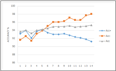
We evaluated our models by varying the number of MB levels L = 2 to 15. The model accuracy on the tuned class steadily rises with the number of levels and flattens at high values of L (Refer to Fig. 5). The behavior is consistent across MBTune(I-ROOT) and MB-Tune-Freeze and across datasets. For binary label MB, the label of an instance is based on which half of the final level it ends up in. For smaller values of L, this decision is based on fewer classifiers and tends to be noisy. We therefore set L = 15 in our experiments.
| Dataset | Test Accuracy % | MB | AMB | AMB- Tune | MB-Tune(I- ROOT) | MB-Tune- Freeze |
|---|---|---|---|---|---|---|
| Spambase | Acc+ | 95.07 | 92.92 | 92.26 | 91.26 (◦3▷6) | 89.83 (◦▷4) |
| Acc-(tuned) | 97.31 | 94.39 | 94.64 | 98.01 (◦▷2) | 97.85 (◦▷1) | |
| Acc | 96.42 | 93.8 | 93.69 | 95.30 (◦1▷5) | 94.66 (◦▷2) | |
| Ionosphere | Acc+ | 91.04 | 83.86 | 83.86 | 92.86 (◦7▷2) | 92.86 (◦7▷2) |
| Acc-(tuned) | 97.72 | 98.66 | 98.66 | 99.27 (◦2▷8) | 99.27 (◦2▷8) | |
| Acc | 96.42 | 93.57 | 93.57 | 97.14 (◦4▷5) | 97.14 (◦4▷5) | |
| Sonar | Acc+ | 89.42 | 87.1 | 85.64 | 92.79 (◦3▷2) | 92.79 (◦3▷2) |
| Acc-(tuned) | 92.27 | 90.33 | 92.44 | 95.81 (◦▷6) | 95.81 (◦▷6) | |
| Acc | 91.08 | 88.67 | 88.91 | 94.37 (◦1▷1) | 94.37 (◦1▷1) | |
| Liver | Acc+(tuned) | 85.87 | 79.32 | 84.11 | 87.72 (◦2▷9) | 82.75 (◦3▷6) |
| Acc- | 71.77 | 55.86 | 43.69 | 74.19 (◦7▷0) | 73.68 (◦6▷7) | |
| Acc | 81.65 | 70 | 72.46 | 82.59 (◦4▷0) | 78.98 (◦4▷1) | |
| Splice* | Acc(rest) | 96.05 | - | - | 95.96 | 95.67 |
| Acc(tuned) | 97.43 | - | - | 98.39 | 98.27 | |
| Acc | 96.39 | - | - | 96.55 | 96.40 | |
| Iris* | Acc(rest) | 89.19 | - | - | 89.19 | 86.48 |
| Acc(tuned) | 95.65 | - | - | 100 | 91.30 | |
| Acc | 91.67 | - | - | 93.33 | 88.33 |
5.6 Run Time Analysis
Table 3 shows the average run time (in ms) to build 15 levels of MB. Evaluation was done on an Intel i7 machine with 8GB RAM and a 64-bit OS. Interactive MB indeed takes longer to train. We believe it could be improved either by appropriate grouping of features to limit the number of hyperparameters or by a multi-threaded implementation. As expected, MBTune-Freeze takes lesser time to train due to early freezing of nodes, with only marginal impact on the accuracy (as seen in Table 2). We believe that our interactive MB model with the option of early freezing might be an acceptable choice especially for large datasets.
| MB | MB-Tune(I- ROOT) | MB-Tune- Freeze | |
|---|---|---|---|
| Spambase | 1009 | 29394 | 27880 |
| Ionosphere | 288 | 1050 | 1030 |
| Sonar | 230 | 623 | 422 |
| Liver | 496 | 949 | 936 |
| Granularity (#Tuned) | Acc+ | Acc- | Acc | |
|---|---|---|---|---|
| Spambase | I-ROOT | 93.80 | 93.27 | 93.48 |
| I-ALL (6) | 93.12 | 94.37 | 93.86 | |
| I-SELECT (3) | 92.86 | 93.97 | 93.22 | |
| I-ROOT | 88 | 96.67 | 93.57 | |
| Ionosphere | I-ALL (6) | 90.71 | 97.72 | 95.41 |
| I-SELECT (2) | 90.71 | 96.84 | 94.66 |
5.7 Effect of Granularity of User Interaction
We grew a 4-stage martingale boosting program and interactively tuned the learner at every node (I-ALL), with the intent of achieving a reduction in false positives. We compare its performance (Refer Table 4) with the one interactively tuned only at the root node (I-ROOT). Although IROOT does automatically tune other nodes, I-ALL benefits from the interactive refinement at all nodes and does better in meeting user preferences. In an attempt to check how many user interactions significantly affect the accuracy, we selectively tuned nodes (I-SELECT), where the advantage is below certain threshold (set to 0.3). Combined with our node freezing strategy, this further reduces the number of nodes requiring manual tuning. On UCI Spambase and Ionosphere, the number of nodes requiring manual tuning in I-SELECT reduced by a factor of 2 and 3 respectively as compared to I-ALL. Since the manual effort for our interactive MB model is a function of the number of nodes tuned, we believe that I-SELECT might significantly reduce the effort with little impact on model accuracy.
6 Conclusion
We presented an approach and a system called interactive martingale boosting for multiclass classification. Our approach attempts to meet user preferences on the performance of a classifier through interactive tuning of a martingale boosting-based classifier. We showed its effectiveness against other approaches through evaluation on several datasets. We also studied the trade-off between human effort and accuracy using interaction at different granularity in the MB program.
Acknowledgments
This research at IIT Bombay was supported through the IBM Faculty Award.
@inproceedings{ijcai2016p124,
  title     = {Interactive Martingale Boosting},
  author    = {Kulkarni, Ashish and Burange, Pushpak and Ramakrishnan, Ganesh},
  booktitle = {Proceedings of the Twenty-Fifth International Joint Conference on
               Artificial Intelligence, {IJCAI-16}},
  publisher = {AAAI Press / International Joint Conferences on Artificial Intelligence},
  editor    = {Subbarao Kambhampati},
  pages     = {841--846},
  year      = {2016},
  month     = {7},
  url       = {https://ijcai.org/proceedings/2016/124},
}
TY - CPAPER TI - Interactive Martingale Boosting AU - Kulkarni, Ashish AU - Burange, Pushpak AU - Ramakrishnan, Ganesh T2 - Proceedings of the Twenty-Fifth International Joint Conference on Artificial Intelligence, IJCAI-16 PB - AAAI Press / International Joint Conferences on Artificial Intelligence PY - 2016 SP - 841 EP - 846 UR - https://ijcai.org/proceedings/2016/124 ER -Copied
Machine-readable versions of this paper, for tools and AI agents:





