Interactive Scheduling of Appliance Usage in the Home

1 Introduction

Demand-side management (DSM), whereby energy demand is controlled by using incentives and automation, is one of the key foci within the domain of Smart Grid [Department of Energy & Climate Change, 2009a; 2009b]. In particular, the concept of DSM can be explained as follows: By minimising the peaks in energy consumption, it reduces the need for expensive peaking plants that are typically highly carbon intensive. Thus it is expected to have a major impact on CO2 emissions and overall generation costs, particularly to the domestic sector, where energy consumption accounts for approximately 27% of the total worldwide energy usage [IEA, 2009].

State-of-the-art DSM solutions typically follow the concept of agent-based demand-side management, which have been proposed to perform complex calculations in order to obtain an optimal plan that maximises consumers' savings [Vytelingum et al., 2011; Ramchurn et al., 2011b]. In particular, this concept involves deploying autonomous software agents in smart meters in homes, acting on the behalf of the users. By taking into account the real time carbon content (or cost of electricity), each agent can schedule the appliance usage in order to minimise peak demand. However, these techniques typically do not consider users' preferences during schedule planning. This can lead to unfortunate cases when the proposed plan is rejected due to the fact that they are not convenient to the users. For example, suppose that a user prefers to use the washing machine on weekends when they have time to take the clothes out to dry and iron them. Consequently, they are likely to reject any suggestions to use the washing machine on a weekday, even it may be cheaper to do so. Thus, solutions recommended by existing methods will not be acceptable to users when they are not compatible with their everyday routine. Since the main goal is to minimise the consumption peaks, we cannot achieve this if the users consistently reject the recommended plans. Given this, we argue that it is essential to take into account the user's preferences as well as the user's typical consumption patterns in the home when scheduling loads.

While machine learning approaches can be efficiently used to learn the usage profile of homeowners in a non-intrusive manner [Truong et al., 2013; Parson et al., 2012], these methods do not learn which appliances are deferrable within a particular user profile, and therefore, cannot provide optimal recommendations other than the current schedule. As such, systems that can learn the user preferences in an interactive way are more desired 1 . For example, some notable work in this area uses static elicitation techniques to learn the user's preferences [Trabelsi et al., 2015]. In particular, these systems typically ask users a number of preset questions (e.g., preferred times). Other works use alerts and notification messages to provide communication between user and agent [Costanza et al., 2014].

However, the main drawback of these approaches is that they do not take into account the bother cost, that is, the cost of making the user feeling annoyed, that occurs during the interaction with the user. In particular, in order to recommend a more efficient scheduling plan that accurately takes into account the user's preferences and total saving cost, preference elicitation systems typically interact with a user in a repeated manner (e.g., asking a series of questions, or sending many alerts and recommendation messages). However, previous work has shown that too many interaction requests (e.g., high number of elicitation questions) will significantly increase the bother cost [Fleming and Cohen, 2004; Ren et al., 2007]. As a consequence, the system will become more intrusive, which will make it less user friendly, and thus, will not be widely applied in homes. On the other hand, an insufficiently low level of interaction (e.g., fewer questions, or less recommendation messages) will lead to an inaccurate and inefficient (i.e., low cost saving) scheduling plan, that is likely to be rejected by the user. Therefore, it is essential to find an efficient balance between having low bother cost and successful information elicitation.

1 In this paper, by interactivity, we refer to methods that proactively learn user profiles through a communication interface.

Since the DSM literature does not provide solutions that can efficiently handle this trade-off, this paper aims to fill this gap in the following way. We propose an interactive preference elicitation based scheduling system, iDR (for interactive Demand Response), that provides efficient trade-offs between (i) non-intrusiveness and accurate information elicitation; and (ii) cost savings and the user's convenience (derived from the learnt preferences). In particular, our solution is inspired by a novel adaptive preference elicitation model [Baarslag and Gerding, 2015], which relies on Pandora's Rule [Weitzman, 1979], a powerful sequential decision-making process. In more detail, iDR works as follows: it first applies a stateof-the-art appliance usage prediction model [Truong et al., 2013] to predict the usage profile of appliances within the upcoming period. It then uses the adaptive elicitation model based on Pandora's Rule to calculate the optimal amount of required interactions (e.g., the number of alert and suggestion messages, or the number of questions to ask). In particular, at each elicitation round, Pandora's Rule first identifies whether to continue the interaction with the user. If further interactions are needed, the elicitation model will calculate the next optimal interaction step to execute (e.g., which alert message to send, or which question to ask). Based on the collected information (i.e., the outcome of the interaction), iDR solves a non-trivial combinatorial optimisation problem to a schedule the appliance usage, which efficiently balances between user convenience and monetary saving. Next, it recommends the calculated schedule to the user, and observes whether it is acceptable. In case it is rejected, iDR proceeds with the next elicitation round. This repeated interaction enables iDR to update the user preference model in real time. Moreover, it allows to select personalised recommendations that strike the balance between savings and convenience, while maintaining a minimal user bother cost. Given this, we advance the state of the art in the following way:

• ÷ We propose iDR, the first interactive demand side management mechanism for scheduling appliance usage, that incorporates appliance usage prediction, combinatorial optimisation, and intelligent user preference elicitation, to improve users' savings and convenience, while still maintains the low level bother cost of the system. Furthermore, our work is a first step towards building more human-aware AI systems that can learn user preferences to schedule their personal activities.
• ÷ We demonstrate through extensive empirical evaluation, using a well-known real-world dataset, that iDR indeed helps users saving more (by up to 35%), while maintaining the balance of user comfort and bother cost, compared to other non-trivial benchmarks.

2 ProblemDescription

This section provides the formal description of the interactive appliance usage scheduling problem. To do so, we first introduce the following notations. Suppose that we have a finite set of appliances, A, that will be used in the next time period, which is discretised by a sequence of time slots 1↪ 2↪ ▷ ▷ ▷ ↪ T (e.g., consider a day ahead scheduling with T = 24). For now, we assume that A is given. In fact, we can identify A by using any appliance usage prediction methods (see Section 3 for more details). For each a 2 A and t = 1↪ 2↪ ▷ ▷ ▷ ↪ T, we denote by xa(t) = ¶0↪ 1♦ the usage of appliance a at time slot t; that is, xa(t) = 1 if a is used at time slot t, and xa(t) = 0 otherwise 2 . Let S = ¶xa(t)♦a↪t denote a usage schedule of the appliances (with a and t running over all the possible values), and let S denote the set of all possible schedules. As mentioned earlier, we aim to maximise the cost saving of the user, while minimising the bother cost and maintaining a good level of user convenience. To achieve this, we define an objective function that includes all of these goals. As such, we first start with the definition of the main terms of the objective function, namely: the consumption cost, user convenience, and user bother cost.

Consumption cost: Now, suppose that the user uses appliance a at time slot t. The (monetary) cost of this usage is calculated as follows:Ca(t) = dacap(t) (1)

where da is the duration of operation for appliance a (in hours), ca is the power consumption of appliance a (in kW), and p(t) is the electricity price at time t (in £/kWh). In our model, we assume that we know the value of p(t) for each t (e.g., we have access to the dynamic pricing scheme of the prices from the electricity providers). Given this, the total consumption cost of schedule S is defined as:

User convenience: Ideally we want to identify the optimal S that minimises Eq. (2). However, this schedule itself does not take into account the need for convenience of the user. As a consequence, it would be rejected by the user. To overcome this issue, we introduce the concept of convenience, which then can be taken into account during the recommendation, as follows:

Our model assumes that the user already has some appliance usage patterns, which is represented by schedule S0 2 S.

2 For the sake of simplicity, we only consider appliance usage as a binary function. However, our model can be extended to other cases, when the same appliance can be used multiple time within one time slot. the only change we need to make is to apply different optimisation tools in Section 3.

The intuition behind this is that homeowners typically deploy the system into their home, where some kind of usage pattern has already been set up, which might not be optimal (hence the goal of the system is to identity a better schedule). In case there exists multiple possible existing patterns, we set S0 to be the one with the maximum likelihood probability 3 . For each pair of schedules S1 = ¶x1(t)♦ and S2 = ¶x2(t)♦, we define the discrepancy between them as follows:

That is, D(S1↪ S2) measures the (L1) distance between the two schedules. As such, we can then define the user's inconvenience as a function of D(S↪ S0). More formally, we have:

where f(·) is a monotone increasing function of D(S↪ S0) (i.e., the larger is the discrepancy, the higher the inconvenience level of the user).

User bother cost: As discussed in Section 1, considering only consumption cost and user convenience is not sufficient to successfully recommend usage schedules to the user (i.e., without rejection). In particular, it is likely that there are other hidden preferences that form constraints for the schedule optimisation problem (e.g., the user prefers to use the washing machines at the weekend, or using the ovens between 7pm and 9pm). To elucidate these hidden preferences, we rely on an interactive preference elicitation approach. However, this approach comes with a cost, namely the intrusiveness, which is measured by the user bother cost as follows.

Suppose that the interaction consists of rounds, at each of which the system can gain some additional information about the user. We denote by Q the set of interactions from which the system can choose to interact with the user at each round r. Suppose that qr is the chosen interaction type at round r, and let o(qr) denote the outcome of interaction type qr (e.g., the information gained after using qr, or the concrete response of the user). In addition, we denote by Hr-1 = ¶q1↪ q2 ▷ ▷ ▷ ↪ qr-1♦ the history of total interactions up to before round r. Given this, let B(Hr-1↪ qr) denote the user bother cost, that is, the cost of having the user interacting with the system. Note that the user bother cost can depend on many parameters, such as the difficulty of the interaction, and the time required to interact. In our model, we consider the following bother cost model:

where B(pr♣Hr-1) is the bother cost of having qr interaction at round r, given the history Hr-1 of previous interactions. This model is reasonable, as it assumes that each interaction has its own bother cost, which, however, depends on the previous interactions.

Objective function: Given the definition of the three components, we now turn to the description of our objective function. In particular, we aim to identify the following optimal schedule and interaction scheme:

3 This probability can be calculated by our appliance usage prediction algorithm (see Section 3 for more details).

where HR denote the total history of interaction during the process. That is, we want to find an optimal interaction scheme H⇤R and a schedule S⇤ that maximises savings, while minimising the user inconvenience and bother cost. Note that C(S) - C(S0) denotes the monetary saving by moving from S0 to S. The reason we use this in the objective function, instead of solely relying on C(S), is that S0 can change over time (as usage patterns change). Thus, our objective function can always adapt to these changes. Both coefficients ↵ and β play a normalisation role here 4 .

3 The Interactive Demand Response System

Given the definition of the objective function, we now turn to the description of our approach. In particular, we first discuss a sequential decision making model, the Pandora Problem, which forms a basis of our solution. We also describe Pandora's Rule, an optimal solution to the Pandora Problem. We then show how we build our preference elicitation algorithm, based on Pandora's Rule. Finally we describe the whole workflow of our system.

3.1 The Pandora Problem

The Pandora Problem was introduced in [Weitzman, 1979], and can be described as follows: Consider N boxes, each of which contains a reward (e.g., gold) with an unknown value. However, we know the distribution of each reward. Let random variable Xk denote the reward of box k. Our goal is to open the box with the highest reward value. However, to open each box k, we have to pay a certain cost ck. During the process, we can subsequently open a number of boxes, and when we stop, we receive the highest reward from the opened boxes, and we have to pay the total cost of openings (i.e., the sum of opening costs). This is a sequential decision making problem, where at each round, we have to decide whether to continue opening the boxes, and if yes, then which one. Our goal is then to find an optimal box opening strategy with an optimal stopping policy (i.e., when to stop opening).

To solve this problem, [Weitzman, 1979] has proposed the following algorithm, called Pandora's Rule. To understand this optimal algorithm, we first introduce some notations. Let Fk(x) denote the cumulative distribution function of Xk for each k. For each box k, let zk denote the solution of the following equation:

where ck is the cost of opening box k. The value zk is called the reservation price of box k, which has the following informal meaning: Suppose that somebody offers us a guaranteed reward of zk independently from the content of box k, and opening box k would only gain us benefit if the reward in box k is larger than zk. In this case, if zk is the solution of Eq. (6), then there is no benefit from opening box k (as the expected extra reward, the right hand side of Eq. (6), is equal to the cost of opening).

4 In fact, this is a linear combination of multiple objectives: we both want to maximise savings and minimise user inconvenience.

Now, Pandora's Rule works as follows: For each box, we calculate its reservation price zk. In the first round, we open the box with the highest reservation price, and we store the observed reward with parameter Xmax (this parameter stores the current highest observed reward). For each subsequent round r, we check whether the current highest observed reward, denoted by Xmax , is higher than the highest reservation price of the remaining (i.e., unopened) boxes. If it is the case, then we stop and the received reward is the current value of Xmax , otherwise we open the box with highest reservation price, and we proceed to round r + 1.

Weitzman has proved that this algorithm is optimal in terms of maximising the expected return (i.e., the highest observed reward). In what follows, we will demonstrate how to tailor this method to the interactive preference elicitation problem.

3.2 Pandora based Preference Elicitation

Recall that at each elicitation round r, the way of interaction is chosen from the set Q. Let qr denote the chosen interaction form, and let o(qr) denote the observed response of the user. Based on the response and history Hr-1, let S(o(qr)↪Hr-1) denote the set of feasible schedules (that do not violate the user's preferences). In addition, for each schedule S, we define its utility values as U(S) = C(S) - C(S0) - ↵I(S). Given this, we identify the best schedule possible, after using qr as the interaction form, denoted by S⇤ (qr), as follows:

Now, if we consider the interaction forms are boxes, then choosing qr from Q corresponds to opening a box, with the reward value of the box equal to S⇤ (qr). Indeed, note that the value of S⇤ (qr) depends on o(qr) (i.e., the outcome of qr), which is unknown before the interaction (i.e., before opening the box). Thus, we can consider S⇤ (qr) as a random variable. In addition, recall that choosing interaction form qr comes with a bother cost B(pr♣Hr-1), which corresponds to the cost of box opening. Finally, our original objective function can be rephrased as maximising the utility of the schedule (i.e., maximising the reward from the opened boxes), minus the total bother cost (i.e., total bother cost). Thus, there is a clear mapping from our problem to Pandora's Problem.

However, note that there is a significant difference between our problem and the Pandora model. In particular, in Pandora's Problem, the costs of opening the boxes are fixed over time. On the other hand, our bother cost model assumes that the bother cost of each interaction form qr also depends on the history, and thus, can change over time. Due to this difference, Pandora's Rule is not guaranteed to be optimal over the course of multiple interactions, as the proof of optimality in [Weitzman, 1979] relies on the fact that the costs are fixed over time. Nevertheless, as we will show in Section 4, the Pandora based elicitation model still provides good performance in our setting.

3.3 TheWorkflow of iDR

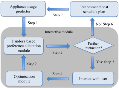
Given the Pandora based elicitation approach, we now turn to the description of the iDR system. In particular, the workflow of iDR is depicted in Figure 1, and can be detailed as follows:

We first use an appliance usage prediction method to infer information about the set A of possible appliances which will be used in the next T time steps (Step 1). In our model, we rely on the graphical model based approach from [Truong et al., 2013]. This prediction method use historical data of appliance usage to estimate the interdependencies between the usage of different appliances, and thus, can make an accurate prediction for future usage. Note that in case historical data is available only in an aggregated energy consumption form (i.e., we do not have which appliances were used in the past, but only the aggregated total energy consumption profile of the household), we can use the energy usage disaggregation model of [Parson et al., 2012] to estimate the usage profile of each appliances. Note that both techniques are non-intrusive, and thus, do not induce any user bother costs.

Having the set of usable appliances A, iDR then uses the Pandora based elicitation model to decide whether further interaction with the user is required (Step 2). If the model requires further interactions, then iDR applies Pandora's Rule to choose which interaction type will be used (Step 3). From the response of the user, iDR employs its optimisation module to identify the best usage schedule, taking into account the constraints learned from the interactions with the user (Step 4). Our model uses off-the-shelf optimisation algorithms within this module. As such, due to page limitations, we do not go into the details of this module. Note that after the calculations, the optimisation module also sends the results to the elicitation module (Step 5), so the latter can update its value for the next elicitation round (see previous section for more details). Conversely, if the elicitation module decides to stop interacting with the user (Step 6), the system provides its final recommendation, which is the best schedule so far, to the user. At the end of the process, all the gathered information (through the interactions with the user) will be shared with the usage prediction model as well (Step 7), so that the latter can update its knowledge about the usage profile of the homeowner, and thus, can improve its future prediction accuracy.

4 Empirical Evaluation

So far we have described iDR, a general framework that enables us to balance between savings maximisation, convenience maintenance, and user bother cost minimisation. In this section, we provide a proof of concept by demonstrating how iDR works in a specific scenario by implementing iDR to a concrete environment and show how it is superior to its benchmarks. To do so, we first discuss a concrete scenario in which iDR is deployed in Section 4.1. We then describe the benchmark strategies that we use to compare against our approach (Section 4.2). Finally, we discuss how iDR performs on a real-world dataset, compared to the benchmarks.

4.1 Experimental Setup

This section provides the description of the settings of relevant components for our experiment: We first describe the appliance settings and the dataset taken from a real-world application, based on which we implement our simulation environment. We then discuss a concrete interaction framework we implemented for testing iDR. We then provide a simulation model of the user's decision-making process to mimic user interactions within the system. We also define the user's bother cost function for this concrete scenario.

Dataset and Appliances

We run our experiments on the Reference Energy Disaggregation Data Set (REDD) [Kolter and Johnson, 2011], which includes electrical usage data from six different houses. These houses had been monitored for approximately 35 days with sub-meters installed on multiple relevant electrical home appliances (e.g, washing machine, dish washer, dryer). The raw data in the REDD dataset contains power consumption of appliances with a granularity of 3 seconds. We converted the raw data to a list of cyclic on-off events; i.e., a list of tuples happliance, start time, end timei. To evaluate our iDR system, we use house 1 in the REDD dataset, as we observed that this house has the most detailed data. We use 75% of the REDD dataset as a training set, and the remaining 25% as a test set. This dataset allows us to apply the appliance usage prediction algorithm from [Truong et al., 2013] to predict the set of appliances A, which will be used each day across the testing dataset. We are also able to identify the typical current schedule S0 is the homeowner.

To evaluate the performance of our strategy under reasonable real-time pricing schemes, we simulate real-time energy prices as proposed by [Ramchurn et al., 2011a]. 5 To calculate the energy usage for each appliance, we apply the average of real data collection on the appliance usage's duration and their energy consumption collected from multiple sources. 6

5 The approach generates the prices from simulated aggregate demand on the grid.

6 For example, a dishwasher typically requires approximately 1.85 (kWh) in 2 hours of operation, while a washing machine consumes around 0.63 (kWh) in 1.5 hours on average. Source: http://www.daftlogic.com/information-appliancepower-consumption.htm.

Question based Preference Elicitation

In our experiments, we implemented a question based interaction interface for preference elicitation. The reason behind this choice is its simplicity. However, note that our system works for any other types of interactions, such as suggestion message based, or scheduling tables [Costanza et al., 2014]. Nevertheless, we find this question based interface to be sufficient to demonstrate the efficiency of iDR. In particular, the system asks binary questions from, or send suggestions to, the user, such as: "Would you like to turn on your washing machine at 7pm instead?", or "Do you think delaying the usage of the kettle by 1hr would be fine?". The intuition of using binary questions/suggestions is that it simplifies the number of possible answers the user can give, which requires simpler user response and bother cost models (see the next two sections for more details). On the other hand, more complex question types will lead to the necessity of deeper psychological knowledge of user response and bother cost models, which is out of scope of this paper.

User Response

In an ideal scenario, the user would say "yes" with probability 1 to any questions or suggestions that have positive total utility(i.e., the combination of savings and convenience) for them, and "yes" with probability 0 (i.e., "no") to any suggestions that have negative total utility. This is equivalent to a step function applied to the total utility. However, even if we assume our model of user responses is completely correct (i.e., that their decision boundary between comfort and savings is linear), people do not always behave rationally very near to their decision boundary (i.e., occasionally, they may say 'no' to perfectly good suggestions) [Costanza et al., 2014]. To improve the realism of our model of user responses, we use logistic regression as our decision-making model for how users deal with given suggestions. More practically, it is more convenient to perform logistic regression with differentiable functions (which the step function is not), and the sigmoid function is by far the most widely used function for this purpose in settings that have binary classifications [Bishop, 2006]. Formally speaking, let qr denote the binary suggestion, and o(qr) is the response of the user, with o(qr) = 1 to be "yes" and "no" otherwise. Let S0 denote the current schedule the user is following, and S1 is the new schedule if o(qr) = 1. We apply a sigmoid function within the user utility function given in Eq 7 to model user responses to suggestions qr. Then, the likelihood of the user to accept a suggestion qr can be estimated as a sigmoid function as follows:

where U(S) is the utility value of schedule S, defined in Section 3.2. Using this sigmoid function, it is thus possible to simulate the user responses to the agent's suggestions. To obtain the user's decision on the system's elicited questions, we selected ↵ = 1 for the marginal comfort cost, as this is indicative of a typical user who is willing to make a trade-off between comfort and cost. We did, however, run our simulations for different values of ↵ and found the relative ranking of our approach and benchmarks is unaffected by this choice.

Bother Cost Function

In our setting, we assume that given a particular history of interactions, all the suggestions have the same bother cost. The intuition behind this is that since all the questions/suggestions are simple and binary, their bother cost do not differ from each other, as they typically require the same cognitive process to answer. However, we also assume that the increased number of elicitation questions may increase the user's bother cost per question as well. For the sake of simplicity, we apply a linear relationship between the current question's bother cost and the number of previously asked questions in our experiment. 7 More formally, we have: For any Hr-1 history and pr qr pair of questions:

where λ is a unit bother cost, and ♣Hr-1♣ is the number of questions elicited so far across the day 8 .

4.2 Benchmark Algorithms

In our experiments, we use two benchmark elicitation strategies to compare against our strategy:

• ÷ Random algorithm (Rand): An agent elicits an offer at random at every round of user's elicitation process. This can be considered as a baseline strategy. For the rest of the process (i.e., appliance usage prediction and optimisation), this algorithm still uses the state of the art.
• ÷ Best Savings (BS): An agent elicits a number of offers that have the highest expected utility (i.e., the combination of savings and convenience) among all incoming offers. Similar to the previous benchmark, this algorithm also applies the state of the art to the rest of the process. Compared to our algorithm, this technique will be greedy on utility.

7 Note that iDR does not rely on the choice of the bother cost function. In fact, we have also run a number of experiments with other types of bother cost functions, such as constant, sublinear (e.g., logarithmic), or exponential. All show a similar broad view.

8 In our experiments shown in Section 4.3, for the sake of simplicity, we set λ = 1 and we vary the value of β (the normalisation coefficient of the bother cost in the objective function) instead.

The intuition of using these benchmarks is as follows: with Rand, we aim to demonstrate that preference elicitation is indeed required. In particular, by ignoring the additional information that could be gained through an intelligent elicitation process, the overall outcome of the system will be very low. On the other hand, BS represents a class of algorithms that focuses on utility maximisation, while bother cost is handled in a greedy manner. As we will show in the next section, both benchmarks are significantly outperformed by iDR.

4.3 Numerical Results

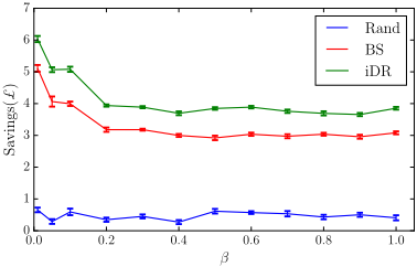
Figure 2 shows the monetary savings performed by the algorithms with different bother costs. We varied the bother cost's coefficient value β to evaluate the performance of each system. Note that the higher the β value, the higher the bother cost. To compare savings between our approach against other benchmarks, we use the same number of elicitation questions on every algorithm each day. By doing so, the bother cost of different approaches can be similar each day. To do so, we first ran iDR to obtain the number of questions that will be elicited to the user during the day, for each β value. Since only iDR can specify when the system should stop eliciting user's preference across the day, while other benchmarks do not. Then, we ran the benchmark algorithms with the same number of elicitation questions obtained by iDR. The results are given for N = 100 rounds. We can clearly see iDR significantly dominated all others across all elicitation costs. In particular, iDR outperformed BS system, the second best, about up to 35%. As expected, we obtained a better pay-off for lower costs, and peaks at closed to zero costs, particularly in the crucial interval [0, 0.2] for β value. The performances are converged gradually when the bother cost is increased (i.e., β > 0▷2) because the number of elicitation questions will stay the same.

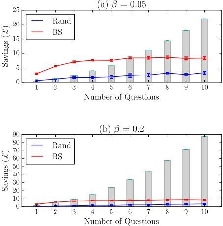
To explain why we use the same number of questions to compare the performance of our approach against others, we run our benchmarks with a different number of elicitation questions each day (Figure 3). As we clearly see that by increasing the number of questions, the benchmarks produce exponentially higher bother costs, while savings is not increased at all. Thus, without an efficient trade-off, these algorithms would provide insufficient performance. On the other hand, iDR can derive the optimal number of questions. Thus, by providing the optimal number of questions to the benchmarks, we are actually making them more efficient within our comparison.

5 Conclusions

We introduced iDR, an interactive appliance usage scheduling system, that can efficiently balance between savings maximisation, user convenience maintenance, and bother cost minimisation. To do so, we combined a novel Pandora based preference elicitation approach with state-of-the-art appliance usage prediction and optimisation tools. We demonstrated, using real-data based simulations, that our system indeed outperforms the existing benchmarks by achieving up to 35% more savings, while user bother cost kept at a minimum level. As a next step, we aim to run field experiments where we apply our system to real homes, with real users.