
Towards Fast Algorithms for the Preference Consistency Problem Based on Hierarchical Models
Proceedings of the Twenty-Fifth International Joint Conference on Artificial Intelligence. Pages 1081-1086.
Abstract
In this paper, we construct and compare algorithmic approaches to solve the Preference Consistency Problem for preference statements based on hierarchical models. Instances of this problem contain a set of preference statements that are direct comparisons (strict and non-strict) between some alternatives, and a set of evaluation functions by which all alternatives can be rated. An instance is consistent based on hierarchical preference models, if there exists an hierarchical model on the evaluation functions that induces an order relation on the alternatives by which all relations given by the preference statements are satisfied. Deciding if an instance is consistent is known to be NP-complete for hierarchical models. We develop three approaches to solve this decision problem. The first involves a Mixed Integer Linear Programming (MILP) formulation, the other two are recursive algorithms that are based on properties of the problem by which the search space can be pruned. Our experiments on synthetic data show that the recursive algorithms are faster than solving the MILP formulation and that the ratio between the running times increases extremely quickly.
- [Booth et al., 2010] R. Booth, Y. Chevaleyre, J. Lang, J. Mengin, and C. Sombattheera. Learning conditionally lexicographic preference relations. In ECAI '10, Lisbon, Portugal, August 16-20, 2010, Proceedings, pages 269- 274, 2010.
- [Boutilier et al., 2004] C. Boutilier, R. I. Brafman, C. Domshlak, H. Hoos, and D. Poole. CP-nets: A tool for reasoning with conditional ceteris paribus preference statements. Journal of Artificial Intelligence Research, 21:135-191, 2004.
- [Bräuning and Hüllermeier, 2012] M. Bräuning and E. Hüllermeier. Learning conditional lexicographic preference trees. In Preference Learning (PL-12), ECAI '12 workshop, Montpellier, France, August 28th, 2012, Proceedings, 2012.
- [Bridge and Ricci, 2007] D. Bridge and F. Ricci. Supporting product selection with query editing recommendations. In RecSys '07, Minneapolis, MN, USA, October 19-20, 2007, Proceedings, pages 65-72. ACM, 2007.
- [Dombi et al., 2007] J. Dombi, C. Imreh, and N. Vincze. Learning lexicographic orders. European Journal of Op- erational Research, 183(2):748-756, 2007.
- [Figueira et al., 2005] J. Figueira, S. Greco, and M. Ehrgott. Multiple Criteria Decision Analysis-State of the Art Sur- veys. Springer International Series in Operations Research and Management Science Volume 76, 2005.
- [Flach and Matsubara, 2007] P. A. Flach and E.T. Matsub- ara. A simple lexicographic ranker and probability esti- mator. In ECML '07, Warsaw, Poland, September 17-21, 2007, Proceedings, pages 575-582, 2007.
- [Fürnkranz and Hüllermeier, 2010] J. Fürnkranz and E. Hüllermeier. Preference Learning. Springer-Verlag New York, Inc., New York, NY, USA, 1st edition, 2010.
- [George et al., 2015] A.-M. George, A. Razak, and N. Wil- son. The comparison of multi-objective preference infer- ence based on lexicographic and weighted average models. In ICTAI '15, Vietri sul Mare, Italy, November 9-11, 2015, Proceedings, pages 88-95, 2015.
- [George et al., 2016] A.-M. George, N. Wilson, and B. O'Sullivan. Towards Fast Algorithms for the Prefer- ence Consistency Problem Based on Hierarchical Models (extended version of IJCAI-2016). http://ucc.insight- centre.org/nwilson/PCPalgorithmsProofs.pdf, 2016. Link
- [Liu and Truszczynski, 2015] Xudong Liu and Miroslaw Truszczynski. Learning partial lexicographic preference trees over combinatorial domains. In AAAI '15, Austin Texas, USA, January 2530, 2015, Proceedings, pages 1539-1545. AAAI Press, 2015.
- [Marinescu et al., 2013] R. Marinescu, A. Razak, and N. Wilson. Multi-objective constraint optimization with tradeoffs. In CP '13, Uppsala, Sweden, September 16-20, 2013, Proceedings, pages 497-512, Berlin, Heidelberg, 2013. Springer Berlin Heidelberg.
- [Trabelsi et al., 2011] W. Trabelsi, N. Wilson, D. Bridge, and F. Ricci. Preference dominance reasoning for con- versational recommender systems: a comparison between a comparative preferences and a sum of weights ap- proach. International Journal on Artificial Intelligence Tools, 20(4):591-616, 2011.
- [Wilson and Borning, 1993] M. Wilson and A. Borning. Hi- erarchical constraint logic programming. The Journal of Logic Programming, 16(34):277-318, 1993.
- [Wilson et al., 2015] N. Wilson, A.-M. George, and B. O'Sullivan. Computation and Complexity of Preference Inference Based on Hierarchical Models (extended version of IJCAI-2015). http://ucc.insight- centre.org/nwilson/PrefInfHCLPproofs.pdf), 2015. IJCAI Link
- [Wilson, 2014] N. Wilson. Preference inference based on lexicographic models. In ECAI '14, 18-22 August 2014, Prague, Czech Republic -Including PAIS '14, pages 921- 926, 2014.
References were extracted automatically from the PDF and may contain errors.
Full text extracted automatically from the PDF; figures, tables and equations may differ. The PDF is the version of record.
1 Introduction
In many fields like recommender systems and multi-objective optimization, one wants to reason over user preferences. In these problems, it is often difficult or excessively timeconsuming to elicit all user preferences. The Preference Deduction Problem (PDP) aims at eliciting only few preferences and inferring more preferences from the given ones; this might then be used in a conversational recommender system, for example, to help choose which items to show to the user next [Bridge and Ricci, 2007; Trabelsi et al., 2011]. Typically, an assumption is made on the type of order relation that the user (implicitly) uses to express the preference statements. Such order relations can be, e.g., comparing alternatives by the values of the evaluation functions lexicographically [Wilson, 2014], by Pareto order, weighted sums [Figueira et al., 2005], based on hierarchical models [Wilson et al., 2015] or by conditional preferences structures as CP-nets [Boutilier et al., 2004] and partial lexicographic preference trees [Liu and Truszczynski, 2015]. Here, the choice of the order relation can lead to stronger or weaker inferences and can make solving PDP computationally more or less challenging. In a recommender system or in a multi-objective decision making scenario, the user should only be presented with a relatively small number of solutions, hence, a strong order relation is required. Using PDP based on a lexicographic models has been shown to be successful in reducing the number of solutions, however, computationally can be more expensive. See [Marinescu et al., 2013] and [George et al., 2015] for comparisons between order relations in a multi-objective optimization framework. While PDP based on hierarchical models yields an even lower number of solutions, it is coNP-complete and computationally expensive. The approach taken by the Preference Deduction Problem contrasts with learning a single model that coincides with the user preferences as in [F¨urnkranz and H¨ullermeier, 2010; Dombi et al., 2007; Flach and Matsubara, 2007; Br¨auning and H¨ullermeier, 2012; Booth et al., 2010].
In this paper, we concentrate on another problem that helps solving PDP: the Preference Consistency Problem (PCP). This is the problem of deciding whether given user preferences are consistent, i.e., not contradicting each other. In terms of hierarchical preference models, PCP determines whether there exists a hierarchical model of evaluation functions such that the induced order relation on the alternatives satisfies all preference statements given by the user. For hierarchical preference models, PCP is NP-complete and PCP and PDP are mutually expressible [Wilson et al., 2015], i.e., PCP can be solved directly by solving PDP and vice versa. The main issue in this paper is to find fast algorithms to solve PCP (and thus PDP) for hierarchical models by exploiting the problem's structure and to compare their running times on a set of synthetic data.
The next section gives an introduction to hierarchical preference models, their induced order relation on alternatives, and the Preference Consistency Problem. Section 3 gives a Mixed Integer Linear Programming formulation for PCP that will function as a baseline for our runtime comparisons. Section 4 discusses the exploitation of properties of PCP instances yielding two recursive algorithms. In Section 5, the conducted experiments and their outcome are described. The last section concludes.
A longer version of this paper including proofs and examples is available online [George et al., 2016].
2 The Consistency ProblemBased on Hierarchical Models
For a set of preference statements, consistency is defined to be the property that the statements do not contradict each other. To formally define this term, we first describe the concept of hierarchical models.
2.1 Hierarchical Models
Hierarchical models will from here on be called HCLP models, where HCLP stands for "Hierarchical Constraint Linear Program" and points out the resemblance of the hierarchical order of the evaluation functions in HCLP models to the order of soft constraints in an HCLP [Wilson and Borning, 1993]. In the following, we define HCLP structures, HCLP models, and their implied order relation that is a kind of lexicographic order.
Definition 2.1 (HCLP structures). An HCLP structure is a triple hA↪⊕↪ Ci. Here, A is a finite set of alternatives and C is a set of evaluation functions from the alternatives A to the non-negative rational numbers Q≥0 . ⊕ is an associative, commutative, and strictly monotonic operation on Q≥0 , i.e., x ⊕ y < z ⊕ y if and only if x < z.
In an HCLP structure, the evaluations C as well as their combinations by ⊕ provide ratings of the alternatives due to unfavorable aspects, e.g., costs, for which we assume that 0 is the best value. The notion of HCLP structures was first introduced in [Wilson et al., 2015] with ⊕ as an associative, commutative and monotonic operation. In this paper, we consider ⊕ to be a strictly monotonic operation as this yields interesting properties allowing us to formulate fast algorithms for checking consistency. Furthermore, we assume the operation to be computable in logarithmic time. These assumptions still allow interesting operators like addition and multiplication which seem natural for combining aspects like costs and distances, but strict monotonicity excludes a minimum or maximum operator which could be desired sometimes.
For a subset C ✓ C of evaluations, we define the weak order (transitive and complete binary order) 4⊕C on the set of alternatives in the following way: for ↵↪ β 2 A, ↵ 4⊕C β if and only if Lc2C c(↵) Lc2C c(β). The corresponding strict order ≺⊕C is given by ↵ ≺⊕C β if and only if ↵ 4⊕C β and ↵ 6<⊕C β, i.e., Lc2C c(↵) < Lc2C c(β). Then, the equivalence relation ⌘⊕C is given by ↵ ⌘⊕C β if and only if ↵ 4⊕C β and ↵ <⊕C β, i.e., Lc2C c(↵) = Lc2C c(β). For C = ;, ↵ ⌘⊕C β for all ↵↪ β 2 A.
Definition 2.2 (HCLP models). An HCLP model H for an HCLP structure hA↪⊕↪ Ci is an ordered partition of a subset σ(H) ✓ C of evaluations. We write H as sequence (C1↪ ▷ ▷ ▷ ↪Ck), where the (possibly empty) sets ; ✓ C1↪ ▷ ▷ ▷ ↪ Ck ✓ C are disjoint and Si=1↪▷▷▷↪k Ck = σ(H). We say Ci is the i-th level set in H. We denote the empty HCLP model with σ(H) = ; by H = ().
An HCLP model can be viewed as a hierarchy on the evaluation functions. For HCLP model H = (C1↪ ▷ ▷ ▷ ↪Ck) the level set C1 contains the most important evaluation functions; the level set C2 contains the second most important evaluation functions and so on. Evaluations C ∩ σ(H) that are not included in the HCLP model are irrelevant for rating the alternatives. Accordingly, we compare two alternatives first on a combination by ⊕ of the most important evaluation functions; only if these are equal do we compare them on the combination of the next most important evaluations. Hence, each HCLP model H = (C1↪ ▷ ▷ ▷ ↪ Ck) implies a weak order 4⊕H on the alternatives that is a lexicographic order on combinations of evaluations. More specifically, for two alternatives ↵↪ β 2 A, ↵ 4⊕H β if and only if
- (I) for all i = 1↪ ▷ ▷ ▷ ↪ k, ↵ ⌘⊕Ci β; or
- (II) there exists some i 2 ¶1↪ ▷ ▷ ▷ ↪ k♦ such that ↵ ≺⊕Ci β and for all 1 j < i, ↵ ⌘⊕Cj β.
Similarly to ≺⊕C and ⌘⊕C , we define the strict weak order ≺⊕H and the equivalence relation ⌘⊕H . For ↵↪ β 2 A, ↵ ≺⊕H β if and only if ↵ 4⊕H β and ↵ 6<⊕H β (i.e., condition (II) holds). Analogue, ↵ ⌘⊕H β if and only if ↵ 4⊕H β and ↵ <⊕H β (i.e., condition (I) holds). Note, that by these definitions level sets of HCLP models can be empty, but empty level sets do not affect the relations 4⊕H , ≺⊕H and ⌘⊕H or any statements based on these relations.
In this paper, we consider special classes of HCLP models where the sizes of the level sets are bounded by some constant. The class C(t) is defined to be the set of HCLP models with level sets that contain at most t evaluations, i.e., if H = (C1↪ ▷ ▷ ▷ ↪Ck) is in C(t) then ♣Ci♣ t for all i = 1↪ ▷ ▷ ▷ ↪ k. Note, that the model classes satisfy the relation C(s) ✓ C(t) for s t. Class C(1) contains standard lexicographic models.
Example. Consider the choice of alternatives Apple Pie (AP), Chocolate Cake (CC) and Ice Cream (IC). The desserts are rated by the evaluation functions: calories (c), sugar (s), and fat (f). The values of C = ¶c↪ s↪ f♦ are percentages of the recommended daily intake as shown in Table 1. Here, 0 is the best possible value, meaning 0% sugar, calories or fat of the recommended daily intake is contained in the dessert. Let ⊕ be the standard addition on Q.
| AP | CC | IC | |
|---|---|---|---|
| c | 10 | 13 | 11 |
| s | 23 | 23 | 16 |
| f | 20 | 17 | 24 |
| f s | 43 | 40 | 40 |
f ⊕ s 43
Table 1: Values of c↪ s↪ f↪ f ⊕ s evaluated on AP, CC, IC.
The HCLP model H = (¶f↪ s♦↪ ¶c♦) consists of the pair of most important evaluations f and s followed by the singleton next most important evaluation c. Hence, H is in C(2) but not in C(1). Also, H implies the relations:
IC ≺⊕H CC, since (f(IC) ⊕ s(IC)↪ c(IC)) = (40↪ 11) <lex (40↪ 13) = (f(CC) ⊕ s(CC)↪ c(CC)). Similarly, IC ≺⊕H AP and CC ≺⊕H AP.
2.2 Preference Consistency
In the following, we first describe the language of preference statements considered in this paper and then define PCP. For this, we define LA to be the set of non-strict preference statements ↵ β (meaning ↵ is preferred to β) on alternatives ↵↪ β 2 A. Similarly, LA< is the set of strict preference statements ↵ < β (meaning ↵ is strictly preferred to β) for ↵↪ β 2 A. Let LA = LA [ LA< . We write a preference statement ' 2 LA as ↵' β', and ' 2 LA< as ↵' < β' for ↵'↪ β' 2 A. We denote the non-strict version of preference statements Γ ✓ LA by Γ() , i.e., Γ() = ¶↵' β' ♣ ' 2 Γ♦.
Definition 2.3 (Satisfaction of Preference Statements). Let H be an HCLP model for HCLP structure hA↪ ⊕↪ Ci. We say H satisfies a preference statement ' 2 LA, denoted H ✏⊕ ', if ↵' 4⊕H β' for ' 2 LA ; or ↵' ≺⊕H β' for ' 2 LA< . Furthermore, H satisfies a set of preference statements Γ ✓ LA, denoted H ✏⊕ Γ, if H satisfies all preference statements in Γ, i.e., H ✏⊕ ' for all ' 2 Γ.
Definition 2.4 (Consistency). Let hA↪⊕↪ Ci be an HCLP structure and t 2 ¶1↪ ▷ ▷ ▷ ↪ ♣C♣♦ a constant. We say Γ ✓ LA is C(t)-consistent, if there exists an HCLP model H 2 C(t) such that H ✏⊕ Γ.
It is easy to show that Γ is C(t)-consistent if Γ is C(s)- consistent for some s < t. Also, the empty model H = () always satisfies non-strict statements, but never satisfies strict statements. Thus, Γ ✓ LA is always consistent.
Example (continued). Consider preference statements:
- I strictly prefer ice cream to apple pie (IC< AP).
- I prefer chocolate cake to apple pie (CC AP).
Then (1) is a strict preference statement, (2) is a nonstrict preference statement. As before, HCLP model H = (¶c↪ s♦↪ ¶f♦) satisfies IC ≺⊕H AP and CC ≺⊕H AP and so CC ⪯⊕H AP. Thus, (1) and (2) together are consistent.
We can now formulate the Preference Consistency and Deduction (decision) Problems for classes C(t).
- C(t) Preference Consistency Problem (C(t)-PCP): Given an HCLP structure hA↪ ⊕↪ Ci, a constant t 2 ¶1↪ ▷ ▷ ▷ ↪ ♣C♣♦ and a set of preference statements Γ ✓ LA. Is Γ C(t)-consistent?
- C(t) Preference Deduction Problem (C(t)-PDP): Given an HCLP structure hA↪⊕↪ Ci, a constant t 2 ¶1↪ ▷ ▷ ▷ ↪ ♣C♣♦, some preference statements Γ ✓ LA and ' 2 LA ∩ Γ. Does H ✏⊕ ' hold for all H 2 C(t) with H ✏⊕ Γ?
Wilson et al. [2015] (in their Proposition 1) show that C(t)- PCP and C(t)-PDP are mutually expressive, i.e., PCP can be solved by solving PDP and vice versa:
Proposition 2.5. H ✏⊕ ' for all H 2 C(t) with H ✏⊕ Γ if and only if Γ [ ¶≻'♦ is C(t)-inconsistent, where ≻' = β' < ↵' for ' 2 LA , or ≻' = β' ↵' for ' 2 LA< .
They also established that C(t)-PDP is coNP-complete for any t ≥ 2 (even if ⊕ is strictly monotonic). Thus C(t)-PCP is NP-complete. A greedy algorithm can solve the special cases C(1)-PCP and C(1)-PDP in time O(♣C♣ · ♣Γ♣).
3 MILP Formulation
We describe a Mixed Integer Linear Programming (MILP) formulation for C(t)-PCP with HCLP structure hA↪ ⊕↪ Ci and preference statements Γ ✓ LA, where evaluations C are integral, ⊕ is the standard addition on integers and n = ♣C♣.
Assigning Evaluations to Level Sets: We introduce a matrix of Boolean variables Y 2 ¶0↪ 1♦n⇥n such that yi↪j = 1 if and only if evaluation i is included in the j-th level set of the solution HCLP model. For C(t)-PCP, every evaluation is contained in at most one level set and the cardinality of the level sets is bounded by t.
Maintaining Values of ⊕-combined Level Sets: The matrix of integer variables X 2 Qn⇥♣Γ♣ contains the values of the combined evaluation functions in the level sets for the alternatives of the preference statements. Thus, xi↪' = Lc2Ci c(↵') - Lc2Ci c(β') maintains the degree of support/opposition of statement ' in the i-th level set Ci.
Maintaining the Sign of Level Sets (Supporting, Opposing and Indifferent): The Boolean variables s<0 j↪'↪ s>0 j↪' and s=0 j↪' express the sign for xj↪'. This is, s<0 j↪' = 1 if and only if xj↪' < 0, s>0 j↪' = 1 if and only if xj↪' > 0, and s=0 j↪' = 1 if and only if xj↪' = 0. Since exactly one of the relations holds,
For the implication s<0 j↪' = 1 ) xj↪' < 0, we formulate:
To enforce the equivalences, we make use of the bounds M' and m' and the integrity of the evaluations. In particular, we use that the lowest positive value xj↪' can take is 1 and the highest negative value is -1.
For the implication s>0 j↪' = 1 ) xj↪' > 0, we formulate:
Finally, we enforce s=0 j↪' = 1 ) xj↪' = 0 by
The equivalences follow from (3) together with (4)-(7).
Satisfaction of Strict and Non-strict Statements: Following the definition of 4⊕H , the HCLP model corresponding to the variable assignments of Y satisfies a non-strict statement ' in Γ if and only if
- (I0 ) for all i = 1↪ ▷ ▷ ▷ ↪ n, s=0 i↪' = 1; or
Analogously, a strict statements ' in Γ is satisfied if and only if (II0 ) holds. It is easy to check that conditions (I0 ) or (II0 ) holding for all ' 2 Γ is equivalent to
Inequality (8) yields the satisfaction of Γ() . We enforce satisfaction of all strict statements in Γ, by
The constraints (1)-(9) form a rather simple MILP formulation for C(t)-PCP. Constraints (3)-(9) could be replaced by sums with extreme weights to enforce a lexicographic order on the level sets. However, these inequalities lead to numerical difficulties for the solver. Also, decision variables yi↪j could be substituted by y0i↪j such that y0i↪j = 1 if and only if i is included in a level set ≥ j. Variables s<0 j↪'↪ s>0 j↪'↪ s=0 j↪' 2 ¶0↪ 1♦ might be replaceable by a variable sj↪' 2 ¶0↪ 1↪ 2♦. However, since our MILP is a satisfaction problem, not an optimization problem, it is not clear whether any of these measures improve the formulation. After trying various Constraint Programming models with set or binary variables, different versions of constraints and different search heuristics, the MILP formulation using inequalities (1)-(9) seemed most promising.
4 Recursive Algorithms
In the following, we describe two recursive search algorithms for C(t)-PCP. The algorithms are based on properties of PCP that can be used to prune the search space. Both try to construct a Γ-satisfying HCLP model by sequentially adding new level sets to the model that do not oppose any preference statement that is not strictly satisfied so far. Thus, during the algorithm the current model always satisfies Γ() , the nonstrict version of Γ. We backtrack when the current model cannot be extended further and the model does not satisfy all strict preference statements. The approaches aim to reduce the number of Γ() -satisfying HCLP models constructed by the algorithm. In particular, they try to identify and ignore level sets which cannot lead to a Γ-satisfying HCLP model although not opposing the preference statements.
Utilising Sequences of Singleton Level Sets: The first approach is based on the idea of including as many singleton level sets as possible. This seems computationally less challenging since a Γ() - satisfying sequence of singleton level sets that is maximal in the number of level sets can be found in time O(♣C♣ · ♣Γ♣) [Wilson et al., 2015]. Remember, that Γ() is defined to be the non-strict version of Γ, i.e., Γ() = ¶↵' β' ♣ ' 2 Γ♦. In the following we show that for strictly monotonic operators ⊕ the recursive search algorithm never needs to backtrack over the choice of such singleton sequences. We first establish the following property for strictly monotonic operators ⊕ which can be shown by a short technical proof.
Lemma 4.1. Let ⊕ be a strictly monotonic operator and let X↪ Y ✓ C be sets of evaluation functions with X ✓ Y . Let ↵↪ β 2 A be alternatives such that X is indifferent under ↵ and β, i.e., ↵ ⌘⊕X β. Then ↵ ≺⊕Y β if and only if ↵ ≺⊕Y ∩X β. Hence, ↵ ⌘⊕Y β if and only if ↵ ⌘⊕Y ∩X β.
We define the (non-commutative) combination of two HCLP models H = (C1↪ ▷ ▷ ▷ ↪ Cl) and H0 = (C 01 ↪ ▷ ▷ ▷ ↪ C 0k ) in C(t) as H ◦ H0 = (C1↪ ▷ ▷ ▷ ↪ Cl↪ (C 01 ∩ σH)↪ ▷ ▷ ▷ ↪ (C 0k ∩ σH)), where σH = Si=1↪▷▷▷↪l Ci. It is easy to see that H ◦ H0 is an HCLP model in C(t) as well. The following proposition shows how the satisfaction of preference statements Γ from H0 persists under combination with sequences of singleton level sets that only satisfy Γ() .
Proposition 4.2. Let (hA↪⊕↪ Ci↪ Γ) be an instance of C(t)- PCP. If H = (c1↪ ▷ ▷ ▷ ↪ cl) is a Γ() - satisfying model in C(1) and H0 = (C 01 ↪ ▷ ▷ ▷ ↪ C 0k ) is a Γ-satisfying model in C(t), then H ◦H0 is a Γ-satisfying model in C(t).
Proof. We show, that H ◦H0 satisfies Γ() and strictly satisfies the preference statements that H0 strictly satisfies. Hence, H ◦H0 is a Γ-satisfying HCLP model in C(t).
Recall that a preference statement ' is strictly satisfied when there exists a level set C supporting ', i.e., ↵' ≺C β', and all preceding level sets C 0 are indifferent under ', i.e., ↵' ⌘C0 β'. Hence, the preference statements in Γ that are strictly satisfied by H = (c1↪ ▷ ▷ ▷ ↪ cl) are also strictly satisfied byH◦H0 = (c1↪ ▷ ▷ ▷ ↪ cl↪ (C 01 ∩σH)↪ ▷ ▷ ▷ ↪ (C 0k ∩σH)). Let Γ0 be the set of remaining preference statements that are not strictly satisfied by H. Since H satisfies Γ() , H is indifferent under all statements in ' 2 Γ0 , i.e., ci(↵') = ci(β') for all 1 i l. Consider an arbitrary level set C in H0 and a preference statement ' 2 Γ0 . Repeatedly applying Lemma 4.1 for the singleton level sets in σH \ C yields: ↵' ⇠⊕C β' if and only if ↵' ⇠⊕C∩σH β', where ⇠ is one of the relations ≺, ⌘ or ≻. Thus, the level sets C 0 i ∩σH inH ◦H0 have the same relation towards statements ' 2 Γ0 as the level sets C 0 i in H0 . Since the initial singleton sequence in H ◦ H0 is indifferent under preference statements ' 2 Γ0 , H ◦H0 satisfies ' if and only if H0 satisfies '. Also, all statements Γ ∩ Γ0 are strictly satisfied by H ◦H0 . Hence, H ◦H0 satisfies Γ() and strictly satisfies all statements in Γ that H0 strictly satisfies.
Proposition 4.2 immediately leads to the next result.
Proposition 4.3. Let H be a Γ() -satisfying model in C(1) that consists of a maximal number of singleton level sets. If Γ is C(t)-consistent, then there exists a Γ-satisfying model in C(t) with H as initial sequence.
Based on Proposition 4.3, we describe the algorithm PCcheck that solves C(t)-PCP by trying to construct a Γsatisfying HCLP model. This method is summarised in the algorithm below disregarding the framed parts. After finding an initial singleton sequence (c1↪ ▷ ▷ ▷ ↪ ck) that is maximal while satisfying Γ() (in time O(♣C♣ · ♣Γ♣) by a greedy algorithm [Wilson et al., 2015]), we consider every possible (not opposing) level set C of size 2 ♣C♣ t. Let Γ0 be the set of preference statements in Γ that are not strictly satisfied by H = (c1↪ ▷ ▷ ▷ ↪ ck↪ C). We try to extend the sequence H by another Γ0 -satisfying HCLP model. We construct this extending model by recursively calling the method for the subproblem with statements Γ0 and evaluations C 0 = C-¶c1↪ ▷ ▷ ▷ ↪ ck♦-C. If no such extension exists (that satisfies Γ), we backtrack over the last chosen level set C and try a new level set. Note, that by Proposition 4.3, we never have to backtrack over the choice of singleton level sets, which can be a significant advantage over solving the MILP model. As soon as the currently considered sequence in the algorithm satisfies Γ we stop and return the sequence, i.e., showing that the instance is C(t)-consistent. If no Γ-satisfying sequence can be found after exploiting all possible (Γ() -satisfying) HCLP model, we stop and return that the instance is C(t)-inconsistent.
Maintaining Conflicting Sets: In the following, we extend the algorithm PC-check(C↪ Γ↪ ⊕↪ t) by maintaining conflicting sets that cannot be contained in the later level sets, and thus reduce the number of backtracks. Proposition 4.4 shows that the satisfaction of Γ persists for an HCLP model H0 when combining with an HCLP model H that extends an initial sequence of level sets of H0 by one more level set and only satisfies Γ() .
Proposition 4.4. Let (hA↪⊕↪ Ci↪ Γ) be an instance of C(t)- PCP that is C(t)-consistent. Let H = (C1↪ ▷ ▷ ▷ ↪Ck↪B) be a Γ() -satisfying HCLP model in C(t) and let H0 = (C1↪ ▷ ▷ ▷ ↪Ck↪Ck+1↪ ▷ ▷ ▷ ↪Cl) be a Γ-satisfying HCLP model in C(t) with B ✓ Cj for some k + 1 j l. Then H ◦ H0 = (C1↪ ▷ ▷ ▷ ↪Ck↪B↪Ck+1↪ ▷ ▷ ▷ ↪ (Cj ∩ B)↪ ▷ ▷ ▷ ↪Cl) is a Γ-satisfying HCLP model in C(t).
Proposition 4.4 is proved in a similar way as Proposition 4.2 using Lemma 4.1. Negating the statement yields: If there exists no Γ-satisfying HCLP model in C(t) that extends H, then there exists no Γ-satisfying HCLP model in C(t) that extends (C1↪ ▷ ▷ ▷ ↪Ck) and contains B in some level set. In the second recursive approach, extending the algorithm below by framed parts, we maintain such conflicting sets B. When the algorithm backtracks because no Γ-satisfying extension of the current HCLP model can be found, we mark the last added level set C to be a conflicting set if ♣C♣ s. Then, a new next level set is chosen that does not contain any conflicting set. Although reducing the search space, a potentially exponentially large list of conflicting sets is maintained, where s regulates the space complexity.
| ↵ | | β | | γ | < | δ | |
|---|---|---|---|---|---|---|---|
| c1 | 1 | 0 | 0 | 0 | |||
| c2 | 0 | 2 | 2 | 2 | |||
| c3 | 1 | 1 | 0 | 1 | |||
| c4 | 0 | 2 | 1 | 1 | |||
| c5 | 2 | 0 | 1 | 0 |
Algorithm: PC-check(C↪ Γ↪ ⊕↪ t↪ S = ;↪ s ) H (c1↪ ▷ ▷ ▷ ↪ ck) some Γ() -satisfying singleton sequence with k maximal if H ✏ Γ then return H for all C ✓ C - ¶c1↪ ▷ ▷ ▷ ↪ ck♦ with 2 ♣C♣ t such that there exists no S 2 S with S ✓ C and ↵' 4⊕C β' for all ' with ↵' ⌘⊕H β' do H (c1↪ ▷ ▷ ▷ ↪ ck↪C) if H ✏ Γ then return H else if H ✏ Γ() then Γ0 = ¶' 2 Γ ♣ ↵' ⌘⊕H β'♦, C 0 = C - σ(H) H (c1↪ ▷ ▷ ▷ ↪ ck↪C↪PC-check(C 0 ↪ Γ0 ↪⊕↪ t↪ S↪ s )) if H ✏ Γ then return H else S S [C return InconsistentLet ⊕ be the standard addition on Z. Suppose, in the first step PC-check finds the maximal singleton sequence (c2↪ c1) (which cannot be extended by any other evaluation without violating Γ() ). Then the algorithm will in turn consider sets ¶c3↪ c4♦, ¶c3↪ c5♦, ¶c4↪ c5♦ and ¶c3↪ c4↪ c5♦. The sequences c2↪ c1↪ ¶c3↪ c4♦ and c2↪ c1↪ ¶c4↪ c5♦ violate Γ() . The sequence c2↪ c1↪ ¶c3↪ c5♦ satisfies Γ() but cannot be extended to satisfy Γ. In PC-check(C↪ Γ↪⊕↪ t↪ S↪ s), the set ¶c3↪ c5♦ is added to the conflicting sets S and thus the set ¶c3↪ c4↪ c5♦ does not have to be checked (by Proposition 4.4). PCcheck(C↪ Γ↪⊕↪ t) finds that c2↪ c1↪ ¶c3↪ c4↪ c5♦ violates Γ() . Thus none of the possible sets leads to a Γ-satisfying sequence and "Inconsistent" is returned. Note, that PC-check does not have to backtrack over the choice of evaluations in the initial singleton set sequence c2↪ c1 (by Proposition 4.3).
5 Experimental Runtime Comparisons
In our experiments, we compare the approaches from Section 3 and 4 for solving PCP by their running time. Here, the MILP formulation functions as a baseline and is expected to be outperformed by the two recursive approaches as they directly exploit the problem structure to perform less backtracks in a way that is not recognized by CPLEX. Note, that it is not obvious how to incorporate the pruning of the search space, that is preformed by the recursive algorithms, in a MILP model in form of constraints or heuristics. We investigate the degree of improvement of the recursive algorithms towards the rather simple MILP formulation and the relation of the recursive algorithms towards each other. Though PCcheck(C↪ Γ↪⊕↪ t↪ S↪ s) prunes the search space further than PC-check(C↪ Γ↪⊕↪ t), the list of maintained conflicting sets can grow exponentially large. Thus, it is not obvious if maintaining conflicting sets is advantageous.
Instances: For our experiments we considered different instance sizes, to observe the effect on the running time by varying the number of evaluations n and the number of preference statements g. For the lack of real world data, we generated 50 instances uniformly at random with evaluation functions with domains ¶0↪ 1↪ 2↪ 3↪ 4↪ 5♦ for each of the problem sizes n↪ g 2 ¶10↪ 15↪ ▷ ▷ ▷ ↪ 50♦ where we fix the number of alternatives that the preference statements are based on to m = 25. Note, that not all alternatives generated are involved in preference statements. Thus, m has no direct influence on the size of the search space or the running time. For time reasons, some experiments were not conducted for all instance sizes.
Implementation: We implemented all three approaches in Java Version 1.8 using the IBM ILOG CPLEX (version 12.6.2) library for the MILP formulation. All experiments were conducted independently on a 2.66Ghz quad-core processor with 12GB memory.
We choose ⊕ as the standard addition on the integers. To reduce the number of experiments, we allow the cardinality bound on the level sets to be t = n, the number of evaluations, and fix the cardinality bound on the maintained conflicting sets to s = 5 (which gives the bound ♣S♣ (ns ) (50 5 ) = 2118760). Since C(k0 ) ✓ C(k) for all k0 < k, we expect the running times to be lower for smaller t. Also, C(k) = C(n) for all k ≥ n, i.e., the running times are the same for bigger t. Experimental Results: As expected, solving the MILP formulation of PCP (as presented in Section 3) by the CPLEX solver is much slower than by the two recursive algorithms PC-check (as presented in Section 4), see Table 2. However, it is remarkable how quickly the ratio between the mean times of solving the MILP and PC-check grows with the number of statements and evaluations in the instances.
| g = | n = 10 | n = 15 | n = 20 |
|---|---|---|---|
| PC-check(C↪ Γ↪ ⊕↪ t) | 0.011 | 0.01 | 0.04 |
| 10 PC-check(C↪ Γ↪ ⊕↪ t↪ S↪ s) | 0.003 | 0.01 | 0.03 |
| MILP | 0.22 | 10.53 | 149.81 |
| minimal ratio: MILP/PC-check | 20 | 1053 | 3745.25 |
| PC-check(C↪ Γ↪ ⊕↪ t) | 0.003 | 0.01 | 0.29 |
| 15 PC-check(C↪ Γ↪ ⊕↪ t↪ S↪ s) | 0.001 | 0.01 | 0.28 |
| MILP | 0.22 | 220.28 | >41472 |
| minimal ratio: MILP/PC-check | 73.33 | 22028 | >143006.89 |
The two algorithms PC-check(C↪ Γ↪⊕↪ t) and PCcheck(C↪ Γ↪⊕↪ t↪ S↪ s) show similar behavior of running times for different instance sizes. Figure 1 shows some of the running times for PC-check(C↪ Γ↪⊕↪ t) and PCcheck(C↪ Γ↪⊕↪ t↪ S↪ s). Here, we can see that the running times increase with the number of evaluations n and the number of statements g.
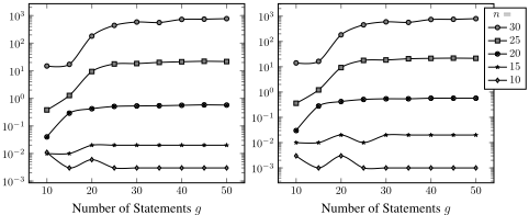
A detailed analysis shows that in 57% of the measured instance sizes PC-check(C↪ Γ↪⊕↪ t) is slower than PCcheck(C↪ Γ↪⊕↪ t↪ S↪ s). The ratios of the mean running times of the two algorithms demonstrate that PC-check(C↪ Γ↪⊕↪ t) is at most 3.67 times slower than PC-check(C↪ Γ↪⊕↪ t↪ S↪ s) and PC-check(C↪ Γ↪⊕↪ t↪ S↪ s) is at most 1.03 times slower than PC-check(C↪ Γ↪⊕↪ t). This insignificant difference between the running times of the two algorithms means that for these instances reducing the number of backtracks by ruling out conflicting sets is not worth the effort and space needed to maintain the list of conflicting sets (of size < 5).
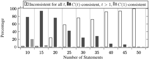
To find an explanation for the behavior of the running times as shown in Figure 1, we observed the occurrence of instances that have solutions in C(1), in C(t) with t > 1, or are inconsistent. The whole search space must be explored until deciding inconsistency for all t, which can lead to high running times. PC-check solves C(1) instances in polynomial time. The instance distribution may suggest that the running times go up with the number of inconsistent instances, e.g., see Figure 2.
6 Conclusion
Exploiting the theoretical results on properties of consistent instances developed in Section 4 allow the algorithms PCcheck to prune the search space much further than a MILP solver could do for the MILP formulation given in Section 3. The experimental results confirm, that the algorithms PCcheck are solving the instances faster than CPLEX. Even more, the ratios between the mean solving times of the MILP and PC-check increase extremely quickly with the number of evaluations and statements. It is not obvious how the pruning rules of the PC-check algorithms can be incorporated in the MILP formulation as constraints.
There is no significant difference between the mean running times of the two recursive algorithms PC-check on the tested instances. Thus, in PC-check(C↪ Γ↪⊕↪ t↪ S = ;↪ s), the effort of maintaining a list S of (possibly exponentially many) conflicting sets to prune the search space further, is not paying off. An analysis of the instance consistency types indicates that the running times for algorithms PC-check might increase with the number of inconsistent instances.
A further analysis could involve the size of the search space, i.e., counting the number of Γ() -satisfying HCLP models and the number of HCLP models that were actually considered during the search. In future work, we will try using a relaxation of a MILP formulation as a fast check for inconsistency within PC-check(C↪ Γ↪⊕↪ t). If the relaxation shows that the current subproblem is inconsistent, we can avoid another (time consuming) recursive call.
Acknowledgment
This publication has emanated from research conducted with the financial support of Science Foundation Ireland (SFI) under Grant Number SFI/12/RC/2289.
@inproceedings{ijcai2016p157,
  title     = {Towards Fast Algorithms for the Preference Consistency Problem Based on Hierarchical Models},
  author    = {George, Anne-Marie and Wilson, Nic and O'Sullivan, Barry},
  booktitle = {Proceedings of the Twenty-Fifth International Joint Conference on
               Artificial Intelligence, {IJCAI-16}},
  publisher = {AAAI Press / International Joint Conferences on Artificial Intelligence},
  editor    = {Subbarao Kambhampati},
  pages     = {1081--1086},
  year      = {2016},
  month     = {7},
  url       = {https://ijcai.org/proceedings/2016/157},
}
TY - CPAPER TI - Towards Fast Algorithms for the Preference Consistency Problem Based on Hierarchical Models AU - George, Anne-Marie AU - Wilson, Nic AU - O'Sullivan, Barry T2 - Proceedings of the Twenty-Fifth International Joint Conference on Artificial Intelligence, IJCAI-16 PB - AAAI Press / International Joint Conferences on Artificial Intelligence PY - 2016 SP - 1081 EP - 1086 UR - https://ijcai.org/proceedings/2016/157 ER -Copied
Machine-readable versions of this paper, for tools and AI agents:





