Change Detection in Multivariate Datastreams: Likelihood and Detectability Loss

1 Introduction

Change detection, namely the problem of detecting changes in probability distribution of a process generating a datastream, has been widely investigated on scalar (i.e. univariate) data. Perhaps, the reason beyond the univariate assumption is that change-detection tests (CDTs) were originally developed for quality-control applications [Basseville et al., 1993], and much fewer works address the problem of detecting changes in multivariate datastreams.

A straightforward extension to the multivariate case would be to independently inspect each component of the datastream with a scalar CDT [Tartakovsky et al., 2006], but this does not clearly provide a truly multivariate solution, e.g., it is unable to detect changes affecting the correlation among the data components. A common, truly multivariate approach consists in computing the log-likelihood of the datastream and compare the distribution of the log-likelihood over different time windows (Section 2). In practice, computing the log-likelihood is an effective way to reduce the multivariate change-detection problem to a univariate one, thus easily addressable by any scalar CDT. Several CDTs for multivariate datastreams pursue this approach, and compute the log-likelihood with respect to a model fitted to a training set of stationary data: [Kuncheva, 2013] uses Gaussian mixtures, [Krempl, 2011; Dyer et al., 2014] use nonparametric density models. Other CDTs have been designed upon specific multivariate statistics [Schilling, 1986; Agarwal, 2005; Lung-Yut-Fong et al., 2011; Wang and Chen, 2002; Ditzler and Polikar, 2011; Nguyen et al., 2014]. In the classification literature, where changes in the distribution are referred to as concept-drift [Gama et al., 2014], changes are typically detected by monitoring the scalar sequence of classification errors over time [Gama et al., 2004; Alippi et al., 2013; Bifet and Gavalda, 2007; Ross et al., 2012].

Even though this problem is of utmost relevance in datastream mining, no theoretical or experimental study investigate how the data dimension d impacts on the change detectability. In Section 3, we consider change-detection problems in Rd and investigate how d affects the detectability of a change when monitoring the log-likelihood of the datastream. In this respect, we show that the symmetric Kullback-Leibler divergence (sKL) between pre-change and post-change distributions is an appropriate measure of the change magnitude, and we introduce the Signal-to-Noise Ratio of the change (SNR) to quantitatively assess the change detectability when monitoring the log-likelihood.

Then, we show that the detectability of changes having a given magnitude progressively reduces when d increases. We refer to this phenomenon as detectability loss, and we analytically demonstrate that, in case of Gaussian random variables, the change detectability is upperbounded by a function that decays as 1◁d. We demonstrate that detectability loss occurs also in non Gaussian cases as far as data components are independent, and we show that it affects also real-world datasets, which we approximate by Gaussian mixtures in our empirical analysis (Section 4). Most importantly, detectability loss is not a consequence of density-estimation problems, as it holds either when data distribution is estimated from training samples or known. Our results indicate that detectability loss is a potentially harmful also at reasonably low-dimensions (e.g., 10) and not only in Big-Data scenarios.

2 Monitoring the Log-Likelihood

2.1 The Change Model

We assume that, in stationary conditions, the datastream ¶x(t)↪ t = 1↪ ▷ ▷ ▷ ♦ contains independent and identically distributed (i.i.d.) random vectors x(t) 2 Rd , drawn from a random variable X having probability-density-function (pdf) φ0, that for simplicity we assume continuous, strictly positive and bounded. Here, t denotes the time instant, bold letters indicate column vectors, and 0 is the matrix transpose operator.

For the sake of simplicity, we consider permanent changes φ0 ! φ1 affecting the expectation and/or correlation of X :

where ⌧ is the unknown change point, v 2 Rd changes the location φ0, and Q 2 O(d) ⇢ Rd⇥d is an orthogonal matrix that modifies the correlation among the components of x. This rather general change-model requires a truly multivariate monitoring scheme: changes affecting only the correlation among components of x cannot be perceived by analyzing each component individually, or by extracting straightforward features (such as the norm) out of vectors x(t)1 .

2.2 The Considered Change-Detection Approach

We consider the popular change-detection approach that consists in monitoring the log-likelihood of x(t) with respect to φ0 [Kuncheva, 2013; Song et al., 2007; Sullivan and Woodall, 2000]:

We denote by L = ¶L(x(t))↪ t = 1↪ ▷ ▷ ▷ ↪ ♦ the sequence of log-likelihood values, and observe that in stationary conditions, L contains i.i.d. data drawn from a scalar random variable. When X undergoes a change, the distribution of L(·) is also expected to change. Thus, changes φ0 ! φ1 can be detected by comparing the distribution of L(·) over WP and WR, two non-overlapping windows of L, where WP refers to past data (that we assume are generated from φ0), and WR refers to most recent ones (that are possibly generated from φ1). In practice, a suitable test statistic T (WP ↪WR), such as the t-statistic, Kolmogorov-Smirnov or Lepage [Lepage, 1971], is computed to compareWP andWR. In an hypothesis testing framework, this corresponds to formulating a test having as null hypothesis "samples in WP and WR are from the same distribution". When T (WP ↪WR) > h we can safely consider that the log-likelihood values over WP and WR are from two different distributions, indicating indeed a change in X . The threshold h > 0 controls the test significance.

There are two important aspects to be considered about this change-detection approach. First, that comparing data on different windows is not a genuine sequential monitoring scheme. However, this mechanism is at the core of several online change-detection methods [Kuncheva, 2013; Song et al., 2007; Bifet and Gavalda, 2007; Ross et al., 2011]. Moreover, the power of the test T (WP ↪WR) > h, namely the probability of rejecting the null hypothesis when the alternative holds, indicates the effectiveness of the test statistic T when the same is used in sequential-monitoring techniques. Second, that φ0 in (2) is often unknown and has to be preliminarily estimated from a training set of stationary data. Then, φ0 is simply replaced by its estimate b φ0. In practice, it is fairly reasonable to assume a training set of stationary data is given, while it is often unrealistic to assume φ1 is known, since the datastream might change unpredictably.

1 We do not consider changes affecting data dispersion as these can be detected by monitoring the Euclidean norm of x(t).

3 Theoretical Analysis

The section sheds light on the relationship between change detectability and d. To this purpose, we introduce: i) a measure of the change magnitude, and ii) an indicator that quantitatively assesses change detectability, namely how difficult is to detect a change when monitoring L(·) as described in Section 2.2. Afterward, we can study the influence of d on the change detectability provided that changes φ0 ! φ1 have a constant magnitude.

3.1 Change Magnitude

The magnitude of φ0 ! φ1 can be naturally measured by the symmetric Kullback-Leibler divergence between φ0 and φ1 (also known as Jeffreys divergence):

This choice is supported by the Stein's Lemma [Cover and Thomas, 2012], which states that KL(φ0↪ φ1) yields an upperbound for the power of parametric hypothesis tests that determine whether a given sample population is generated from φ0 (null hypothesis) or φ1 (alternative hypothesis). In practice, large values of sKL(φ0↪ φ1) indicate changes that are very apparent, since hypothesis tests designed to detect either φ0 ! φ1 or φ1 ! φ0 can be very powerful.

3.2 Change Detectability

We define the following indicator to quantitatively assess the detectability of a change when monitoring L(·).

Definition 1. The signal-to-noise ratio (SNR) of the change φ0 ! φ1 is defined as:

where var[·] denotes the variance of a random variable.

In particular, SNR(φ0 ! φ1) measures the extent to which φ0 ! φ1 is detectable by monitoring the expectation of L(·). In fact, the numerator of (4) corresponds to the shift introduced by φ0 ! φ1 in the expectation of L(·) (i.e., the relevant information, the signal) which is easy/difficult to detect relatively to its random fluctuations (i.e., the noise), which are assessed in the denominator of (4). Note that, if we replace the expectations and the variances in (4) by their sample estimators, we obtain that SNR(φ0 ! φ1) corresponds - up to a scaling factor - to the square statistic of a Welch's t-test [Welch, 1947], that detects changes in the expectation of two sample populations. This is another argument supporting the use of SNR(φ0 ! φ1) as a measure of change detectability.

The following proposition relates the change magnitude sKL(φ0↪ φ1) with the numerator of (4).

Proposition 1. Let us consider a change φ0 ! φ1 such that

where Q 2 Rd⇥d is orthogonal and v 2 Rd . Then, it holds:

Proof. From the definition of sKL(φ0↪ φ1) in (3) it follows

Since L(·) = log (φ0(·)), (6) holds if and only if

From (5) it follows that φ0(x) = φ1(Q0 (x-v)), thus, by replacing the mathematical expectations with their integral expressions, (7) becomes

Let us define y = Q0 (x - v), then x = Qy + v and dx = ♣det(Q)♣dy = dy, since Q is orthogonal. Using this change of variables in the second summand of (8) we obtain

Finally, defining φ2(y) := φ1(Qy + v) turns (9) into

which holds since the left-hand-side of (10) is KL(φ1↪ φ2).

3.3 Detectability Loss

It is now possible to investigate the intrinsic challenge of change-detection problems when data dimension increases. In particular, we study how the change detectability (i.e., SNR(φ0 ! φ1)) varies when d increases and changes φ0 ! φ1 preserve constant magnitude (i.e., sKL(φ0↪ φ1) = const). Unfortunately, since there are no general expressions for the variance of L(·), we have to assume a specific distribution for φ0 to carry out any analytical development. As a relevant example, we consider Gaussian random variables, which enable a simple expression of L(·). The following theorem demonstrates the detectability loss for Gaussian distributions, namely that SNR(φ0 ! φ1) decays as d increases.

Theorem 1. Let φ0 = N(θ0↪⌃0) be a d-dimensional Gaussian pdf and φ1 = φ0(Qx + v), where Q 2 Rd⇥d is orthogonal and v 2 Rd . Then, it holds

where the constant C depends only on sKL(φ0↪ φ1).

Proof. Basic algebra leads to the following expression for L(x) when φ0 = N (θ0↪ ⌃0):

The first term in the right-hand-side of (12) is constant, while the second term is distributed as a chi-squared having d degrees of freedom. Therefore,

Then, from the definition of SNR(φ0 ! φ1) in (4) and Proposition 1, it follows that

Theorem 1 shows detectability loss for Gaussian distributions. In fact, when d increases and sKL(φ0↪ φ1) remains constant, SNR(φ0 ! φ1) is upper-bounded by a function that monotonically decays as 1◁d. The decaying trend of SNR(φ0 ! φ1) indicates that detecting changes becomes more difficult when d increases. Moreover, the decaying rate does not depend on sKL(φ0↪ φ1), thus this problem equally affects all possible changes φ0 ! φ1 defined as in (1), disregarding their magnitude.

3.4 Discussion

First of all, let us remark that Theorem 1 implicates detectability loss only when sKL(φ0↪ φ1) is kept constant. Assuming constant change magnitude is necessary to correctly investigate the influence of the sole data dimension d on the change detectability. In fact, when the change magnitude increases with d, changes might become even easier to detect as d grows. This is what experiments in [Zimek et al., 2012](Section 2.1) show, where outliers 2 become easier to detect when d increases. However, in that experiment, the change-detection problem becomes easier as d increases, since each component of x carries additional information about the change, thus increases sKL(φ0↪ φ1).

Detectability loss can be also proved when φ0 is non Gaussian, as far as its components are independent. In fact, if

2 Even though similar techniques can be sometimes used for both change-detection and anomaly-detection, the two problems are intrinsically different, since the former aims at recognizing process changes, while the latter at identifying spurious data.

φ0(x) = Qdi=0 φ(i) 0 (x(i) ), where (·)(i) denotes either the marginal of a pdf or the component of a vector, it follows

since log(φ(i) 0 (x(i) )) are independent. Clearly, (14) increases with d, since its summands are positive. Thus, also in this case, the upperbound of SNR(φ0 ! φ1) decays with d when sKL(φ0↪ φ1) is kept constant.

Remarkably, detectability loss does not depend on how the change φ0 ! φ1 affects X. Our results hold, for instance, when either φ0 ! φ1 affects all the components of X or some of them remain irrelevant for change-detection purposes. Moreover, detectability loss occurs independently of the specific change-detection method used on the loglikelihood (e.g. sequential analysis, or window comparison), as our results concern SNR(φ0 ! φ1) only.

In the next section we show that detectability loss affects also real-world change-detection problems. To this purpose, we design a rigorous empirical analysis to show that the power of customary hypothesis tests actually decreases with d when data are non Gaussian and possibly dependent.

4 Empirical Analysis

Our empirical analysis has been designed to address the following goals: i) showing that SNR(φ0 ! φ1), which is the underpinning element of our theoretical result, is a suitable measure of change detectability. In particular, we show that the power of hypothesis tests able to detect both changes in mean and in variance of L(·) also decays. ii) Showing that detectability loss is not due to density-estimation problems, but it becomes a more serious issue when φ0 is estimated from training data. iii) Showing that detectability loss occurs also in Gaussian mixtures, and iv) showing that detectability loss occurs also on high-dimensional real-world datasets, which are far from being Gaussian or having independent components. We address the first two points in Section 4.1, while the third and fourth ones in Sections 4.2 and 4.3, respectively.

In our experiments, the change-detection performance is assessed by numerically computing the power of two customary hypothesis tests, namely the Lepage [Lepage, 1971] and the one-sided t-test 3 on data windows WP and WR which contains 500 data each. As we discussed in Section 3.2, the t-statistic on the log-likelihood is closely related to SNR(φ0 ! φ1), while the Lepage is a nonparametric statistic that detects both location and scale changes 4 . To compute the power, we set h to guarantee a significance level 5 ↵ = 0▷05. Following the procedure in Appendix, we synthetically introduce changes φ0 ! φ1 having sKL(φ0↪ φ1) = 1 which, in the univariate Gaussian case, corresponds to v equals to the standard deviation of φ0.

3 We can assume that φ0 ! φ1 decreases the expectation of L since E x⇠φ0 [log (φ0(x))]- E x⇠φ1 [log (φ0(x))] ≥ 0 follows from (7).

4 The Lepage statistic is defined as the sum of the squares of the Mann-Whitney and Mood statistics, see also [Ross et al., 2011].

5 The value of h for the Lepage test is given by the asymptotic approximation of the statistic in [Lepage, 1971].

4.1 Gaussian Datastreams

We generate Gaussian datastreams having dimension d 2 ¶1↪ 2↪ 4↪ 8↪ 16↪ 32↪ 64↪ 128♦ and, for each value of d, we prepare 10000 runs, with φ0 = N(θ0↪⌃0) and φ1 = N(θ1↪⌃1). The parameters θ0 2 Rd and ⌃0 2 Rd⇥d have been randomly generated, while θ1 2 Rd and ⌃1 2 Rd⇥d have been set to yield sKL(φ0↪ φ1) = 1 (see Appendix). In each run we generate 1000 samples: ¶x(t)↪ t = 1↪ ▷ ▷ ▷ ↪ 500♦ from φ0, and ¶x(t)↪ t = 501↪ ▷ ▷ ▷ ↪ 1000♦ from φ1. Then, we compute the datastream L = ¶L(x(t))↪ t = 1↪ ▷ ▷ ▷ ↪ 1000♦, and define WP = ¶L(x(t))↪ t = 1↪ ▷ ▷ ▷ ↪ 500♦ and WR = ¶L(x(t))↪ t = 501↪ ▷ ▷ ▷ ↪ 1000♦.

We repeat the same experiment replacing φ0 with its estimate b φ0(x), where b θ0 and b⌃0 are computed using the sample estimators over an additional training set TR whose size grows linearly with d, i.e. #TR = 100 · d. We denote by bL = ¶ b L(x(t))↪ t = 1↪ ▷ ▷ ▷ ↪ 1000♦ the sequence of estimated log-likelihood values. Finally, we repeat the whole experiments keeping #TR = 100 for any value of d, and we denote

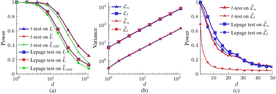
by bL100 the corresponding sequence of log-likelihood values. Figure 1(a) shows that the power of both the Lepage and one-sided t-test substantially decrease when d increases. This result is coherent with our theoretical analysis of Section 3, and confirms that SNR(φ0 ! φ1) is a suitable measure of change detectability. While it is not surprising that the power of the t-test decays, given its connection with the SNR(φ0 ! φ1), it is remarkable that the power of the Lepage test also decays, as this fact indicates that it becomes more difficult to detect both changes in the mean and in the dispersion of L. The decaying power of both tests indicates that the corresponding test statistics decrease with d, which imply larger detection delays when using this statistics in sequential monitoring schemes.

Note that detectability loss is not due to density-estimation issues, but rather to the fact that the change-detection problem becomes intrinsically more challenging, as it occurs in the ideal case where φ0 is known (solid lines). When L is computed from an estimated b φ0 (dashed and dotted lines), the problem becomes even more severe, and worsens when the number of training data does not grow with d (dotted lines).

4.2 Gaussian mixtures

We now consider φ0 and φ1 as Gaussian mixtures, to prove that detectability loss occurs also when datastreams are generated/approximated by more general distribution models. Mimicking the proof of Theorem 1, we show that when d increases and sKL(φ0↪ φ1) is kept constant, the upper-bound of SNR(φ0 ! φ1) decreases. To this purpose, it is enough to show that var [L(x)] increases with d.

x⇠φ0 The pdf of a mixture of k Gaussians is

where λ0↪i > 0 is the weight of the i-th Gaussian N (θ0↪i↪⌃0↪i). Unfortunately, the log-likelihood L(x) of a Gaussian mixture does not admit an expression similar to (12) and two approximations are typically used to avoid severe numerical issues when d ≫ 1.

The first approximation consists in considering only the Gaussian of the mixture yielding the largest likelihood, as in [Kuncheva, 2013] i.e.,

where i⇤ is defined as

The second approximation we consider is:

that is a lower bound of L(·) due to the Jensen inequality.

We consider the same values of d as in Section 4.1 and, for each of these, we generate 1000 datastreams of 500 data drawn from a Gaussian mixture φ0. We set k = 2 and λ0↪1 = λ0↪2 = 0▷5, while the parameters θ0↪1, θ0↪2, ⌃0↪1, ⌃0↪2 are randomly generated. We then compute the sample variance of both Lu and Ll over each datastream and report their average in Figure 1(b). As in Section 4.1, we repeat this experiment by preliminarily estimating b φ0 from a training set containing Ll .

200 · d additional samples, then we compute b Lu and b Figure 1(b) shows that the variances of Lu and Ll grow linearly with respect to d, as in the Gaussian case (13). This indicates that detectability loss occurs also when X is generated by a simple bimodal distribution and, most importantly, also when using Lu or Ll that are traditionally adopted when fitting Gaussian mixtures. As in Section 4.1, we see that loglikelihoods b Lu and b Ll computed with respect to fitted models follow the same trend. We further observe that Ll exhibits a much larger variance than Lu, thus we expect this to achieve lower change-detection performance than Lu.

4.3 Real-World Data

To investigate detectability loss in real-world datasets, we design a change-detection problem on the Wine Quality Dataset [Cortez et al., 2009] and the MiniBooNE Particle Dataset [Roe et al., 2005] from the UCI repository [Lichman, 2013]. The Wine dataset has 12 dimensions: 11 corresponding to numerical results of laboratory analysis (such as density, Ph, residual sugar), and one corresponding to a final grade (from 0 to 10) for each different wine. We consider the vectors of laboratory analysis of all white wines having a grade above 6, resulting in a 11-dimensional dataset containing 3258 data. The Particle dataset contains numerical measurements from a physical experiment designed to distinguish electron from muon neutrinos. Each sample has 50-dimensions and we considered only data from muon class, yielding 93108 data.

In either datasets we have to estimate φ0 for both introducing changes having constant magnitude and computing the log-likelihood. We adopt Gaussian mixtures and estimate k by 5-fold cross validation over the whole datasets, obtaining k = 4 and k = 2 for Wine and Particle dataset, respectively.

We process each dataset as follows. Let us denote by D the dataset dimension and for each value of d = 1↪ ▷ ▷ ▷ ↪ D we consider only d components of our dataset that are randomly selected. We then generate a d-dimensional training set of 200 · d samples and a test set of 1000 samples (datastream), which are extracted by a bootstrap procedure without replacement. The second half of the datastream is perturbed by the change e φ0 ! e φ1, which is defined by fitting at first e φ0 on the whole d-dimensional dataset, and then computing e φ1 according to the procedure in Appendix. Then, we estimate b φ0 from the training set and we compute T (c WP ↪ c WR), where c WP , c WR are defined as in Section 4.1. This procedure is repeated 5000 times to estimate the test power numerically. Note that the number of Gaussians in both e φ0 and b φ0 is the value of k estimated from the whole D-dimensional dataset, and that e φ0 is by no means used for change-detection purposes.

Figure 1(c) reports the power of both Lepage and one-sided t-tests on the Particle dataset, considering b Lu (16) and b Ll (17) as approximated expressions of the likelihoods. The power of both tests is monotonically decreasing, indicating an increasing difficulty in detecting a change among c WP andc WR when d grows. This result is in agreement with the claim of Theorem 1 and the results in the previous sections. The Lepage test here turns to be more powerful than the t-test and this indicates that it is important to monitor also the dispersion of L(·) when using Gaussian mixtures, where L(·) can be multimodal. Moreover, the decaying power of the Lepage test indicates that, as in Section 4.1, monitoring both expectation and dispersion of L(·) does not prevent the detectability loss. Figure 1(c) indicates that b Lu(·) guarantees superior performance than b Ll(·) since this has lower variance than b Lu(·). This fact also underlines the importance of considering the variance of L(·) in measures of change detectability, as in (4). Experiments on Wine dataset, which is approximated by a more sophisticated distribution (k = 4), confirms detectability loss, but the results have not been reported due to space limitations.

We finally remark that have set a change magnitude (sKL(φ0↪ φ1) = 1) that is quite customary in changedetection experiments, as in the univariate Gaussian case this corresponds to setting v equals to the standard deviation of φ0. Therefore, since in our experiments the power of both tests is almost halved when d ⇡ 10, we can conclude that detectability loss is not only a Big-Data issue.

5 Conclusions

We provide the first rigorous study of the challenges that change-detection methods have to face when data dimension scales. Our theoretical and empirical analyses reveal that the popular approach of monitoring the log-likelihood of a multivariate datastream suffers detectability loss when data dimension increases. Remarkably, detectability loss is not a consequence of density-estimation errors - even though these further reduce detectability - but it rather refers to an intrinsic limitation of this change-detection approach. Our theoretical results demonstrate that detectability loss occurs independently on the specific statistical tool used to monitor the log-likelihood and does not depend on the number of input components affected by the change. Our empirical analysis, which is rigorously performed by keeping the changemagnitude constant when scaling data-dimension, confirms detectability loss also on real-world datastreams. Ongoing works concern extending this study to other change-detection approaches and to other families of distributions.

Appendix: Generating Changes of Constant Magnitude

Here we describe a procedure to select, given φ0, an orthogonal matrix Q 2 Rd⇥d and a vector v 2 Rd such that φ1 = φ0(Qx + v) guarantees sKL(φ0↪ φ1) = 1 in the case of Gaussian pdfs, and sKL(φ0↪ φ1) ⇡ 1 for arbitrary distributions. Extensions to different values of sKL(φ0↪ φ1) are straightforward. Since φ1(x) = φ0(Qx + v), we formulate the problem as generating at first a rotation matrix Q such that

and then defining the translation vector v to adjust φ1 such that sKL(φ0↪ φ1) reaches (or approaches) 1.

We proceed as follows: we randomly define a rotation axis r, and a sequence of rotations matrices ¶Qj♦j around r, where the rotation angles monotonically decrease toward 0 (thus Qj tends to the identity matrix as j ! 1). Then, we set Qj ⇤ as the largest rotation yielding a sKL < 1, namely

When φ0 is continuous and bounded (as in case of Gaussian mixtures) it can be easily proved that such a j ⇤ exists.

In the case of Gaussian pdfs, when φ0 = N(θ0↪⌃0), sKL(φ0↪ φ1) admits a closed-form expression:

and sKL(φ0(·)↪ φ0(Qj·)) can be exactly computed to solve (18). When there are no similar expressions for sKL(φ0↪ φ1) this has to be computed via Monte Carlo simulations.

After having set the rotation matrix Q, we randomly generate a unit-vector u as in [Alippi, 2014] and determine a suitable translation along the line v = ⇢u, where ⇢ > 0, to achieve sKL(φ0↪ φ1) = 1. Again, the closed-form expression (19) allows to directly compute the exact value of ⇢ by substituting v = ⇢u into (19). This yields a quadratic equation in ⇢, whose positive solution ⇢⇤ provides v = ⇢⇤u that leads to sKL(φ0↪ φ1) = 1. When the are no analytical expressions for sKL(φ0↪ φ1), we generate an increasing sequence ¶⇢n♦n such that ⇢0 = 0 and ⇢n ! 1 as n ! 1, and set

where sKL(φ0(·)↪ φ0(Q · +⇢nu)) is computed by Monte Carlo simulations. After having solved (20), we determine ⇢⇤ via linear interpolation of [⇢n⇤↪ ⇢n⇤+1] on the corresponding values of the sKL. In this case, we can only guarantee sKL(φ0↪ φ1) ⇡ 1 with an accuracy that can be improved by increasing the resolution of ¶⇢n♦n.