
ADL™: A Topic Model for Discovery of Activities of Daily Living in a Smart Home
Proceedings of the Twenty-Fifth International Joint Conference on Artificial Intelligence. Pages 1404-1409.
Abstract
We present an unsupervised approach for discovery of Activities of Daily Living (ADL) in a smart home. Activity discovery is an important enabling technology, for example to tackle the healthcare requirements of elderly people in their homes. The technique applied most often is supervised learning, which relies on expensive labelled data and lacks the flexibility to discover unseen activities. Building on ideas from text mining, we present a powerful topic model and a segmentation algorithm that can learn from unlabelled sensor data. The model has been evaluated extensively on datasets collected from real smart homes. The results demonstrate that this approach can successfully discover the activities of residents, and can be effectively used in a range of applications such as detection of abnormal activities and monitoring of sleep quality, among many others.
- [Blei and Lafferty, 2007] David M Blei and John D Lafferty. A cor- related topic model of science. The Annals of Applied Statistics, pages 17-35, 2007.
- [Blei et al., 2003] David M Blei, Andrew Y Ng, and Michael I Jor- dan. Latent Dirichlet allocation. Journal of Machine Learning Research, 3:993-1022, 2003.
- [Chen et al., 2012] Liming Chen, Jesse Hoey, Chris D Nugent, Di- ane J Cook, and Zhiwen Yu. Sensor-based activity recognition. Systems, Man, and Cybernetics, Part C: Applications and Re- views, IEEE Transactions on, 42(6):790-808, 2012.
- [Cook et al., 2009] Diane J Cook, M Schmitter-Edgecombe, et al. Assessing the quality of activities in a smart environment. Meth- ods of Information in Medicine, 48(5):480, 2009.
- [Cook et al., 2013] Diane J Cook, Aaron S Crandall, Brian L Thomas, and Narayanan C Krishnan. CASAS: A smart home in a box. Computer, 46(7), 2013.
- [Cook, 2010] Diane J Cook. Learning setting-generalized activity models for smart spaces. IEEE Intelligent Systems, 2010(99):1, 2010.
- [Fleury et al., 2010] Anthony Fleury, Michel Vacher, and Norbert Noury. SVM-based multimodal classification of activities of daily living in health smart homes: sensors, algorithms, and first experimental results. Information Technology in Biomedicine, IEEE Transactions on, 14(2):274-283, 2010.
- [Fowlkes and Mallows, 1983] Edward B Fowlkes and Colin L Mal- lows. A method for comparing two hierarchical clusterings. Jour- nal of the American Statistical Association, 78(383):553-569, 1983.
- [Griffiths and Steyvers, 2004] Thomas L Griffiths and Mark Steyvers. Finding scientific topics. The National Academy of Sciences, 101(suppl 1):5228-5235, 2004.
- [Gu et al., 2010] Tao Gu, Shaxun Chen, Xianping Tao, and Jian Lu. An unsupervised approach to activity recognition and segmenta- tion based on object-use fingerprints. Data & Knowledge Engi- neering, 69(6):533-544, 2010.
- [Hoffman et al., 2010] Matthew Hoffman, Francis R Bach, and David M Blei. Online learning for latent dirichlet allocation. In Advances in Neural Information Processing Systems, pages 856- 864, 2010.
- [Hofmann, 1999] Thomas Hofmann. Probabilistic latent semantic indexing. In The 22nd Annual International ACM SIGIR Con- ference on Research and Development in Information Retrieval, pages 50-57. ACM, 1999.
- [Hong and Nugent, 2013] Xin Hong and Chris D Nugent. Segment- ing sensor data for activity monitoring in smart environments. Personal and Ubiquitous Computing, 17(3):545-559, 2013.
- [Hospedales et al., 2009] Timothy Hospedales, Shaogang Gong, and Tao Xiang. A Markov clustering topic model for mining be- haviour in video. In The 12th International Conference on Com- puter Vision (ICCV-2009), pages 1165-1172. IEEE, 2009.
- [Huynh et al., 2008] Tâm Huynh, Mario Fritz, and Bernt Schiele. Discovery of activity patterns using topic models. In The 10th International Conference on Ubiquitous Computing, pages 10- 19. ACM, 2008.
- [Krishnan and Cook, 2014] Narayanan C Krishnan and Diane J Cook. Activity recognition on streaming sensor data. Pervasive and Mobile Computing, 10:138-154, 2014.
- [Niebles et al., 2008] Juan Carlos Niebles, Hongcheng Wang, and Li Fei-Fei. Unsupervised learning of human action categories using spatial-temporal words. International Journal of Computer Vision, 79(3):299-318, 2008.
- [Ramirez et al., 2012] Eduardo H. Ramirez, Ramon Brena, Davide Magatti, and Fabio Stella. Topic model validation. Neurocom- puting, 76(1):125 -133, 2012.
- [Rosen-Zvi et al., 2004] Michal Rosen-Zvi, Thomas Griffiths, Mark Steyvers, and Padhraic Smyth. The author-topic model for authors and documents. In The 20th Conference on Uncertainty in Artificial Intelligence, pages 487-494. AUAI Press, 2004.
- [Saives et al., 2015] Jérémie Saives, Clément Pianon, and Gregory Faraut. Activity discovery and detection of behavioral deviations of an inhabitant from binary sensors. Automation Science and Engineering, IEEE Transactions on, 12(4):1211-1224, 2015.
- [Salton and Buckley, 1988] Gerard Salton and Christopher Buck- ley. Term-weighting approaches in automatic text retrieval. In- formation Processing & Management, 24(5):513-523, 1988.
- [Toutanova and Johnson, 2007] Kristina Toutanova and Mark John- son. A Bayesian LDA-based model for semi-supervised part-of- speech tagging. In Advances in Neural Information Processing systems, pages 1521-1528, 2007.
- [Vahdatpour et al., 2009] Alireza Vahdatpour, Navid Amini, and Majid Sarrafzadeh. Toward unsupervised activity discovery us- ing multi-dimensional motif detection in time series. In The 21st International Joint Conference on Artificial Intelligence (IJCAI- 2009), volume 9, pages 1261-1266, 2009. IJCAI
- [Van Kasteren et al., 2008] Tim Van Kasteren, Athanasios Noulas, Gwenn Englebienne, and Ben Kröse. Accurate activity recogni- tion in a home setting. In The 10th International Conference on Ubiquitous Computing, pages 1-9. ACM, 2008.
- [Wallach, 2006] Hanna M Wallach. Topic modeling: Beyond bag- of-words. In The 23rd International Conference on Machine Learning (ICML-2006), pages 977-984. ACM, 2006.
- [Wan et al., 2015] Jie Wan, Michael J OGrady, and Gregory MP OHare. Dynamic sensor event segmentation for real-time activity recognition in a smart home context. Personal and Ubiquitous Computing, 19(2):287-301, 2015.
- [Wang and McCallum, 2006] Xuerui Wang and Andrew McCal- lum. Topics over time: a non-Markov continuous-time model of topical trends. In The 12th ACM SIGKDD International Confer- ence on Knowledge Discovery and Data Mining, pages 424-433. ACM, 2006.
- [Wang et al., 2012] Chong Wang, David Blei, and David Hecker- man. Continuous time dynamic topic models. arXiv preprint arXiv:1206.3298, 2012.
- [Wu et al., 2007] Tsu-yu Wu, Chia-chun Lian, and Jane Yung-jen Hsu. Joint recognition of multiple concurrent activities using factorial conditional random fields. In The 22nd Conference on Artificial Intelligence (AAAI-2007), 2007.
- [Wyatt et al., 2005] Danny Wyatt, Matthai Philipose, and Tanzeem Choudhury. Unsupervised activity recognition using automati- cally mined common sense. In The 20th National Conference on Artificial Intelligence (AAAI-2005), volume 5, pages 21-27, 2005.
References were extracted automatically from the PDF and may contain errors.
Full text extracted automatically from the PDF; figures, tables and equations may differ. The PDF is the version of record.
1 Introduction
A smart home is an intelligent residential platform which collects and utilises the diverse data generated in this environment (such as sensor data, video and audio streams) to provide necessary assistance to the residents, especially those who need 24/7 care. The discovery and recognition of Activities of Daily Living (ADL) is an essential function of a smart home: based on the results of this process, the intelligent system can decide which action to take in order to support the residents' well-being. Most existing work in this area has adopted supervised learning to obtain an activity recognition model from smart home data labelled with the current activity. Labelling such data takes time and is error-prone, which motivates the use of unsupervised learning approaches to activity discovery in this paper.
Usually three categories of data for activity discovery/recognition are distinguished [Chen et al., 2012]: (i) visual data, such as video streams of human actions; (ii) data from wearable sensors, used to identify behaviours of a specific actor; and (iii) data collected from environmental sensors. This work concentrates on the latter kind of data, provided by a sensor network consisting of motion sensors, door sensors, light switch sensors, etc. These sensors monitor and record residents' daily activities in several aspects according to their types. Such a sensor network is cheap and easy to set up, with fewer privacy concerns than the other two kinds of sensors.
Topic models are probabilistic models for discovering the hidden structures in a collection of text documents, where the hidden structures can be interpreted as 'topics' described by their most pertinent words. Such models make assumptions about the probability distributions of words, documents and topics, where the first two are observed and the third are hidden or 'latent'. Probabilistic inference can be used to infer the hidden structure, such as the topic distribution for a given document or the probability of a word occurring in particular topics. If we assume that one occurrence of an activity generates one segment of the sensor data, then activities can be viewed as the latent structure underlying this sensor data, which makes topic models a potentially suitable unsupervised approach for activity discovery.
The most significant difference between a text corpus and sensor data is that sensor data does not include splits as occur naturally between words or documents in text data. If we consider activities as 'topics', then we need to abstract 'words' and segment the data into a series of 'documents'. Importantly, we need to model dependencies between time points, which is why in this work we consider bigrams (a sequence of two adjacent elements from a string of tokens) as well as unigrams (one element from a string of tokens) of words.
The approach proposed in this paper hence has the following two ingredients in order to cope with the specifics of sensor data: (i) methods for abstracting words and generating documents from sequential sensor data, which will be introduced in Section 3; (ii) a novel topic model for learning from the documents generated by the first step, which will be described in Section 4. Experimental results will be presented in Section 5.
2 RelatedWork
Several supervised learning approaches to recognition of ADL exist, including temporal models: Hidden Markov Models (HMMs) [Van Kasteren et al., 2008] and Conditional Random Fields (CRFs) [Wu et al., 2007], and point-based classifiers: Support Vector Machines (SVMs) [Fleury et al., 2010] and Na¨ıve Bayes Classifiers (NBCs) [Cook, 2010], etc. In addition to the cost of labelled data, being unable to deal with previously unseen activities is another shortcoming of supervised methods in this area.
Unsupervised approaches include [Saives et al., 2015; Vahdatpour et al., 2009], who mine frequent sub-sequences or motifs of the sequential sensor data. Such methods usually require another learning model (such as clustering models) to categorise the data by means of the discovered patterns. Topic models provide a more robust way to identify patterns that does not require a second model to categorise the data. Other work has applied knowledge-driven approaches for unsupervised activity discovery [Wyatt et al., 2005; Gu et al., 2010], where the idea is to mine relations between objects and activities from the web and then use such information to build learning models. Such methods are limited to sensor data which includes information about specific objects.
Previous work has proposed topic models for learning latent patterns from various kinds of sequential data. Bigram Topic Models (BTMs) [Wallach, 2006] extend the original Latent Dirichlet Allocation (LDA) models [Blei et al., 2003] by replacing unigrams with bigrams. Alternatively, the nonMarkov continuous-time topic model of [Wang and McCallum, 2006] introduces timestamps of words into topic models for discovering topics associated with time. The work in [Niebles et al., 2008] shows how to abstract words and documents from video sequences and apply LDA or probabilistic Latent Semantic Analysis (pLSA) [Hofmann, 1999] for activity recognition. A Markov clustering topic model [Hospedales et al., 2009] introduces an extension of LDA for discovering behaviours in video streams. [Huynh et al., 2008] describes how to apply topic models on wearable sensor data to discover daily routines. These works suggest that topic models might be beneficial for discovery of ADL from environmental sensors as well.
Modelling streaming data often requires segmented data for learning. The most common idea is to use sliding windows, usually consisting of a fixed number of time points [Krishnan and Cook, 2014]. For supervised learning, each window is a data point and its aggregate properties form the features. This is not suitable for topic models, since if we treat each window as a document then the difference between adjacent documents is just one time point. [Hong and Nugent, 2013] and [Wan et al., 2015] proposed several segmentation methods for labelled sensor data without sliding windows: the main idea is to utilise the correlation between sensors, locations and activities to decide which point could be a split of the data. For unlabelled data, the information of activities is absent, but the mapping between sensors and locations are still available.
These previous works suggest that topic models could be a feasible unsupervised approach for discovering and recognising activities from sensor data. Our approach is presented in the following sections.
3 SensorWords and Sensor Documents
Words and documents are the building blocks of text-based topic models. Hence, the first step is to define words and documents in the context of sensor data. Data used in our experiments are obtained from the CASAS project 1 which are partially annotated. The format of the sensor data is illustrated in Table 1. Many sensors, such as motion sensors, door sensors and light switches, provide binary readings, whereas others provide continuous values, e.g. temperature sensors. Since the latter are more closely related to environmental factors than ADL, in this work we focus on binary sensors. We combine the sensor identifier and the sensor reading into one "word", which allows us to transform the sensor data into a sequence of words. For M binary sensors we obtain a vocabulary with 2M unique words.
| Timestamp | Sensor | Reading | Activity |
|---|---|---|---|
| 2013-04-01 00:04:09.340911 2013-04-01 00:04:10.485392 2013-04-01 00:56:31.879063 2013-04-01 01:13:53.616434 . . . 2013-04-01 02:45:47.215554 | M007 M007 T106 BATV104 . . . M006 | ON OFF 24 3070 . . . OFF | Sleep Begin Sleep End |
As for sensor documents, ideally each of them corresponds to one specific activity (topic). We hence need to segment the continuous sensor data into activity-related documents. As suggested in [Hong and Nugent, 2013], locations of a smart home are highly correlated with specific activities. We hence consider a change of location as a strong signal of a switch between activities. This cannot be a fully accurate mapping since people are likely to move around when they are doing something. To fix this, we require segments to be of a min-
1 http://ailab.wsu.edu/casas/datasets.html
Algorithm 1: Document Segmentation Algorithm Input : Ls - the sequence of sensor locations, terminated with an extra 0, and all location IDs are non zero. Input : tth - time threshold Output: Docs - the list of start and stop indices of each document 1 Docs = /0; 2 idxstart =0; 3 idxstop = idxstart ; 4 while idxstop < len(Ls)-1 do 5 idl =Ls[idxstop] ; 6 idxstop = idxnext -1, where idxnext is the next index that satisfies Ls[idxnext ] 6= idl ; 7 tstop = timestamp of Ls[idxstop]; 8 tstart = timestamp of Ls[idxstart ]; 9 if tstop-tstart > tth then 10 append (idxstart ↪ idxstop) into Docs; 11 idxstart = idxnext ; 12 end 13 idxstop = idxnext ; 14 end 15 return Docs;imum duration, expressed by the time threshold tth. If one location is only visited briefly, the data will not be split until the next location change occurs. The algorithm is given in Algorithm 1. This algorithm can be easily converted to an online version for activity recognition in real-time by adding a second time threshold to limit the maximum duration of a document.
4 A Topic Model for Discovery of ADL
This section describes the topic model we propose for discovery of Activities of Daily Living, which is called ADL TM . Each document in this model is treated as a combination of unigram and bigram words. In this way, ADL TM can categorise the documents not only by activations of single sensors but also by transitions between different sensors.
4.1 Generative Process
As we expect that each document of the sensor data is generated by one activity in our settings, in the generative process of ADL TM all words of a document are drawn from the same topic. As shown in the graphical probabilistic model we adopt for ADL TM (Figure 1), there are two independent word sequences composing one document: (i) a sequence of unigrams which are independently drawn; (ii) a sequence of bigrams which are represented by a Markov chain.
In this probabilistic model K is the number of topics, D is the number of documents, M is the number of unigrams in document d, N-1 is the number of bigrams in document d. In theory, the unigrams and bigrams of this model could be from different vocabularies, so the lengths of the two sequences are not necessarily the same. For instance, if we want to categorise documents not only by sensors but also by time information, we could define hours of timestamps of
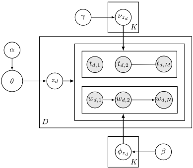
1 Draw a q ⇠Dir(a); 2 for d =1 to D do 3 Draw a topic zd ⇠Multi(q); 4 Draw a fzd ⇠Dir(b); 5 Draw a nzd ⇠Dir(g); 6 for n = 1 to N do 7 Draw a unigram td↪n♣zd ⇠ Mult(nzd ); 8 if n > 1 then 9 Draw a bigram wd↪n♣wd↪n-1↪ zd ⇠ Mult(fzd ); 10 end 11 enddata points as unigrams instead, thus the discovered topics can take into account time as well. When td↪i and wd↪i are the same, M is equal to N and V is equal to H. In this simplified scenario, the generative process of ADL TM is as specified in Algorithm 2.
Unlike Latent Dirichlet Allocation (LDA) [Blei et al., 2003], topics are drawn for documents rather than words in this model. The topic zd of document d is drawn from a multinomial distribution Mult(q), where q is drawn from a symmetric Dirichlet distribution Dir(a). A unigram td↪i is conditioned on topic zd and drawn from a multinomial distribution Mult(nzd ), where nzd is a H-dimensional vector drawn from a symmetric Dirichlet distribution Dir(g), and H is the size of the unigram vocabulary. Bigrams are denoted as wd↪i♣wd↪i-1 and are also conditioned on the topic zd, so they are drawn from a multinomial distribution Mult(fzd ) where fzd is a V ⇥V matrix and V is the vocabulary size of wd↪i.
4.2 Gibbs Sampling of ADL TM
An effective approximation approach to inference in topic models is Gibbs sampling [Rosen-Zvi et al., 2004; Griffiths and Steyvers, 2004], which is one of the most popular Markov Chain Monte Carlo algorithms. The core idea of Gibbs sampling is to construct the Markov chain by drawing each latent variable from their conditional distribution in turn. In Gibbs sampling of ADL TM , the conditional probability of topic zd can be estimated as follows:
where z-d represents topics assigned to all documents except document d, t-d and w-d are unigram and bigram sequences of all other documents except document d. As a topic is drawn for each document, the joint probability of topics of all documents can be calculated by:
Since zd ⇠Multi(q) and q ⇠Dir(a), the first term of Equation (1) can be estimated by:
where Ck is the number of documents assigned to topic k except current document d.
As all words in a document are drawn from one topic, the full conditional probability of the bigram sequence wd can be estimated by Equation (4), where I(x) is the indicator function; wd↪n is the n th word in the bigram sequence of document d; Cwi jk is the number of times word j is followed by word i in topic k, except in current document d; and Cw⇤ jk is the number of times word j followed by any word in topic k, except in current document d.
An important characteristic of the sensor data is that most transitions between sensors are self-transitions. If we want to estimate the probability of transitions between different sensors in an activity, which is the purpose of introducing bigrams, the weights of self-transitions should be decreased in probability estimation. A common approach in natural language processing is to use tf -idf [Salton and Buckley, 1988] as the weight of each individual word. tf indicates term frequency which is simply defined as the number of times a word appears in the dataset. idf refers to the inverse document frequency, where the document frequency is the number of documents that contain this word. When the term frequency is much higher than the document frequency, tf -idf is still dominated by term frequency, so in this case we deployed document frequency for counting bigrams in Equation (4).
Similarly, all the unigrams in document d are drawn together too, so the conditional probability of td is given by:
where Cthk is the number of times the unigram h has been assigned to topic k, except in document d; and Ct⇤k is the number of times that any unigram has been assigned to topic k, except in document d. Here, unlike for bigrams, the counts of unigrams are counted by term frequency.
Using Equations (3) to (5), the probability P(zd♣z-d↪w↪ t) (Equation (1)) can be calculated by Gibbs sampling and subsequently the parameters q , f , n of ADL TM can be estimated.
5 Experimental Evaluation
We have tested our approach on several CASAS datasets which were collected in real smart homes. The properties of datasets hh122, hh120 [Cook et al., 2013] and milan [Cook et al., 2009] are listed in Table 2. These datasets are partially annotated with activities, so this gives us an opportunity to compare the results of our unsupervised model with the annotations. All test results in this section are produced with the following hyperparameters:
- Topic prior: a =50◁K;
- Bigram and unigram priors: b = 5◁V , g = 5◁H.
The number of topics K is guaranteed larger than the number of locations and selected by several tests, because we assume there are more types of activities than locations. However, if K is too large there will be empty topics (which are not assigned any document) after convergence. For instance, there are 9 locations of dataset hh122, so K is experimentally set to 12. The number of iterations of Gibbs sampling is 50.
5.1 Evaluation of Discovered Topics
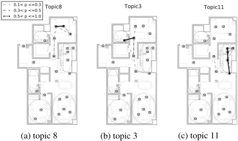
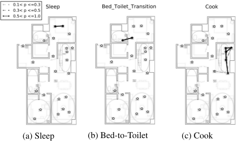
To understand what hidden patterns have been discovered by ADL TM , we have visualised the discovered topics. As illustrated in Figure 2, the most frequently activated sensors and transitions of a topic (the black dots and lines) only appear in one location. This phenomenon matches the actual activities, which mostly occur in a specific location of the house: for example, "Sleep" occurs in the bedroom and "Cook" occurs in the kitchen. Although some sensors of neighbouring locations are also involved, they are much less frequent in that topic (grey dots and lines). Compared with the annotated activities (Figure 3), these discovered topics are similar but somewhat less concentrated in an area.
| Dataset | # Activities | # Binary Sensors | Duration (days) | # Residents |
|---|---|---|---|---|
| hh122 | 32 | 24 | 30 | 1 |
| hh120 | 32 | 24 | 64 | 1 |
| milan | 15 | 31 | 31 | 1+pet |
| hh122 | hh120 | milan | |
|---|---|---|---|
| Random topics | 0.0798 | 0.0969 | 0.1193 |
| BTM | 0.1515 | 0.1988 | 0.3225 |
| LDA | 0.3268 | 0.3486 | 0.5634 |
| ADL TM | 0.3362 | 0.4072 | 0.6190 |
To evaluate the similarity between discovered topics and annotated activities, we adopted the Fowlkes-Mallows (FM) Index [Fowlkes and Mallows, 1983; Ramirez et al., 2012], a variant of the F1 score adapted for clustering, to measure the discovered topics quantitatively. The results on three datasets are shown in Table 3, which indicates ADL TM outperforms LDA [Blei et al., 2003] and BTM [Wallach, 2006] in this criterion.
5.2 Evaluation of Segmentation
Another thing worth evaluating is the segmentation by topics. After the documents have been categorised by topics, new segments of the data sequence are generated. Some adjacent documents assigned to the same topic have been merged together and become a new segment now. In the ideal case, each segment of topics should correspond to one occurrence of the resident's daily activities. We evaluate the segmentation by several metrics as described in this section.
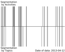
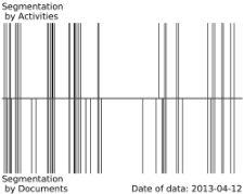
Figure 4 displays segmentation by activities, topics and documents. They are visualised with one day's data. The discovered topics integrate some documents so that the segments become less trivial but meanwhile additional error might occur due to the integration.
We have defined two criteria to evaluate the segmentation quantitatively:
(b) Segmentation by documents and activities
Figure 4: Visualisation of segmentation by ADL TM (dataset: hh122). The upper half of a sub-figure is the segmentation by activities, lower half is by topics (a) or documents (b). The date at the bottom right is the date when the data was generated.
- Segmentation Error, which is the average error over all segments of the data sequence:
where Ds is the number of generated segments in the data sequence; Ndp is the total number of data points; and Ei is the number of data points in segment i who do not belong to the dominant activity of this segment, which can be calculated as
Here, Ni denotes the number of data points in segment i; ai j is the annotated activity of data point j in segment i; I(x) is the indicator function; m is the activity that has maximum number of data points in segment i.
- Fragment Ratio, which is the average number of segments in one occurrence of an activity:
where Da is the number of occurrences of activities in the evaluated data.
The segmentation by actual activities is viewed as the ideal result with segmentation error zero and fragment ratio one.
Table 4 gives the evaluation results of segmentation by different methods tested on three datasets. The documents are generated by the algorithm described in Algorithm 1. As we can see, the documents have lower segmentation errors and higher fragment ratio than the topic models, because most of the documents are much smaller than segments of activities or topics. The topic models decrease the fragment ratio by integrating trivial documents but increase the segmentation error. The results show that ADL TM outperforms LDA [Blei et al., 2003] and the BTM [Wallach, 2006] in both criteria.
The topic segmentation is based on the document segmentation, so the parameter tth of the segmentation algorithm (Algorithm 1) can affect the segmentation results of topic models as well. When tth is smaller, the segmentation error is lower, the fragment ratio is higher and vice-versa, resulting in a trade-off between the two criteria when choosing this parameter. Hence in practical cases some prior knowledge about the minimum duration of activities will help to improve the segmentation results.
| hh122 | hh120 | milan | ||||
|---|---|---|---|---|---|---|
| Errs | Rf r | Errs | Rf r | Errs | Rf r | |
| Documents | 0.0197 | 1.596 | 0.0404 | 2.084 | 0.0342 | 1.563 |
| LDA | 0.0541 | 1.178 | 0.0531 | 1.554 | 0.0409 | 1.157 |
| BTM | 0.0619 | 1.174 | 0.0568 | 1.853 | 0.0428 | 1.394 |
| ADL TM | 0.0512 | 1.102 | 0.0516 | 1.364 | 0.0406 | 1.149 |
(b) Distribution of "Sleep"
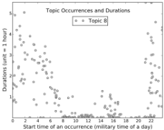
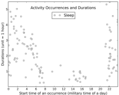
Figure 5: Topic 8 and Annotated Activity Sleep (dataset: hh122). The x-axis indicates the start time of a segment and the y-axis gives the duration of a segment in hours.
5.3 Applications
After the documents have been categorised by topics the data sequence is fully segmented and a new data space can be constructed by generating one data point for each segment with 3 features: the start time-stamp of its segment, the duration and the topic of this segment. By this transformation, the raw data space is highly compressed without losing important information: for instance, the dataset hh122 is compressed from 129936 to 2792 data points. Based on the compressed data space, we can perform various further analyses to leverage information contained in the discovered topics.
As can be seen in the visualisation of topic 8 (Figure 2a), we can assume that it represents the bedroom activities, so now we visualise all the segments assigned to topic 8 as in Figure 5a. The data points with duration larger than 1 hour are mostly distributed between 10 PM to 7 AM, which indicates the regular sleeping time of the resident during night. We can also easily calculate the average sleeping duration of this resident as 7.02 hours. When combined with the distribution of topic 3 (Figure 2b), we can infer that the resident usually needs to use the toilet 3 times per night during sleep. Figure 5b plots the annotated activity "Sleep". These two figures are very similar, which indicates that the discovered topic 8 successfully represents the activity "Sleep".
However, not all topics map to one specific activity: e.g. activities in the kitchen are usually divided into breakfast, lunch and dinner activities, which can be distinguished by the time of their occurrences. As the discovered topic 11 (Figure 2c) corresponds to kitchen activities, a very simple but effective approach to obtain those sub-topics is K-means clustering. The only feature we need is the start time of a segment, and the number of clusters K is set to 3. To examine how accurate the clustering result is we mapped the annotated kitchen activities to the discovered sub-topics as in Table 5. The subtopics successfully represent breakfast, lunch and dinner activities and the categorisation is quite precise.
| Sub- Topic | Cook Breakfast | Wash Breakfast Dishes | Cook Lunch | Wash Lunch Dishes | Cook Dinner | Wash Dinner Dishes |
|---|---|---|---|---|---|---|
| 0 | 0.985 | 0.904 | 0 | 0 | 0 | 0 |
| 1 | 0 | 0 | 0 | 0 | 0.969 | 0.979 |
| 2 | 0 | 0.041 | 0.960 | 0.983 | 0 | 0 |
| Timestamp | Sensor | Reading | Location |
|---|---|---|---|
| 2013-04-27 18:29:28.187573 | MA011 | ON | Kitchen |
| 2013-04-27 18:29:29.339714 | MA011 | OFF | Kitchen |
| 2013-04-27 20:47:55.930002 | M010 | ON | Kitchen |
| 2013-04-27 20:47:57.065529 | M010 | OFF | Kitchen |
We can also easily detect outliers by deploying z-scores on the duration of all data points of a topic. In this way, one outlier of kitchen activities has been detected in dataset hh122. The corresponding raw data points are shown in Table 6: between the two sensors switching on then off no other sensor activations have occurred during more than 2 hours, which is clearly an abnormal situation.
6 Conclusions and FutureWork
In this paper we proposed a topic model ADL TM and a segmentation algorithm for discovery of Activities of Daily Living in a smart home. It is a novel unsupervised approach for modelling sequential sensor data, thus sidestepping the expensive requirement of providing labelled training data. Successful unsupervised methods are a crucial step in making activity discovery feasible in practice. Our experimental results have demonstrated that discovered topics can represent actual activities successfully and work effectively in various practical applications. The segmentation of the data is also close to the true segments with a low level of error. ADL TM outperforms Latent Dirichlet Allocation (LDA) [Blei et al., 2003] and the Bigram Topic Model (BTM) [Wallach, 2006] in both criteria of the topic-activity similarity and segmentation evaluations.
There are several avenues for future work. Simultaneously categorising data by spatial as well as temporal dimensions could enhance the clustering performance, some ideas have been introduced in topic models for document categorisation [Wang and McCallum, 2006][Wang et al., 2012]. Secondly, in order perform incremental discovery of new topics, an online extension of the model is required, which for efficiency would require an online variational inference algorithm as used for standard LDA [Hoffman et al., 2010]. Thirdly, since a small part of labelled data could provide prior knowledge that can be used for estimating hyperparameters and for mapping topics to actual activities, it is also worth extending the model to allow semi-supervised learning[Toutanova and Johnson, 2007]. Finally, correlations between topics could be introduced into the model, following ideas proposed in [Blei and Lafferty, 2007] and [Hospedales et al., 2009].
Acknowledgments
This work was performed under the a Sensor Platform for HEalthcare in a Residential Environment (SPHERE) Interdisciplinary Research Collaboration funded by the UK Engineering and Physical Sciences Research Council, Grant EP/K031910/1.
@inproceedings{ijcai2016p202,
  title     = {ADL™: A Topic Model for Discovery of Activities of Daily Living in a Smart Home},
  author    = {Chen, Yu and Diethe, Tom and Flach, Peter A.},
  booktitle = {Proceedings of the Twenty-Fifth International Joint Conference on
               Artificial Intelligence, {IJCAI-16}},
  publisher = {AAAI Press / International Joint Conferences on Artificial Intelligence},
  editor    = {Subbarao Kambhampati},
  pages     = {1404--1409},
  year      = {2016},
  month     = {7},
  url       = {https://ijcai.org/proceedings/2016/202},
}
TY - CPAPER TI - ADL™: A Topic Model for Discovery of Activities of Daily Living in a Smart Home AU - Chen, Yu AU - Diethe, Tom AU - Flach, Peter A. T2 - Proceedings of the Twenty-Fifth International Joint Conference on Artificial Intelligence, IJCAI-16 PB - AAAI Press / International Joint Conferences on Artificial Intelligence PY - 2016 SP - 1404 EP - 1409 UR - https://ijcai.org/proceedings/2016/202 ER -Copied
Machine-readable versions of this paper, for tools and AI agents:





