
Robust Domain Generalisation by Enforcing Distribution Invariance
Proceedings of the Twenty-Fifth International Joint Conference on Artificial Intelligence. Pages 1455-1460.
Abstract
Many conventional statistical machine learning algorithms generalise poorly if distribution bias exists in the datasets. For example, distribution bias arises in the context of domain generalization, where knowledge acquired from multiple source domains need to be used in a previously unseen target domains. We propose Elliptical Summary Randomisation (ESRand), an efficient domain generalisation approach that comprises of a randomized kernel and elliptical data summarisation. ESRand learns a domain interdependent projection to a latent subspace that minimises the existing biases to the data while maintaining the functional relationship between domains. In the latent subspace, ellipsoidal summaries replace the samples to enhance the generalisation by further removing biasand noise in the data. Moreover, the summarization enables large-scale data processing by significantly reducing the size of the data. Through comprehensive analysis, we show that our subspace-based approach outperforms state-of-the-art results on several activity recognition benchmark datasets, while keeping the computational complexity significantly low.
- [Bengio et al., 2007] Yoshua Bengio, Pascal Lamblin, Dan Popovici, Hugo Larochelle, et al. Greedy layer-wise train- ing of deep networks. In Proceedings of Advances in Neural Information Processing Systems (NIPS), volume 19, pages 153-160, 2007.
- [Bezdek et al., 2011] James C Bezdek, Sutharshan Ra- jasegarar, Masud Moshtaghi, Christopher Leckie, Marimuthu Palaniswami, and Timothy C Havens. Anomaly detection in environmental monitoring networks. IEEE Computational Intelligence Magazine, 6(2):52-58, 2011.
- [Blanchard et al., 2011] Gilles Blanchard, Gyemin Lee, and Clayton Scott. Generalizing from several related classifi- cation tasks to a new unlabeled sample. In Proceedings of Advances in Neural Information Processing Systems (NIPS), pages 2178-2186, 2011.
- [Blum, 2006] Avrim Blum. Random projection, margins, ker- nels, and feature-selection. In Proceedings of Subspace, Latent Structure and Feature Selection, pages 52-68. 2006.
- [Erfani et al., 2015] Sarah M. Erfani, Mahsa Baktashmotlagh, Sutharshan Rajasegarar, Shanika Karunasekera, and Chris Leckie. R1SVM: a Randomised Nonlinear Approach to Large-Scale Anomaly Detection. In Proceedings of Associ- ation for the Advancement of Artificial Intelligence (AAAI), pages 432-438, 2015.
- [Erfani et al., 2016a] Sarah M Erfani, Mahsa Baktashmot- lagh, Sutharshan Rajasegarar, Vinh Nguyen, Christo- pher Leckie, James Bailey, and Kotagiri Ramamohanarao. R1STM: One-class Support Tensor Machine with Ran- domised Kernel. In Proceedings of SIAM International Conference on Data Mining (SDM), 2016.
- [Erfani et al., 2016b] Sarah M. Erfani, Sutharshan Ra- jasegarar, Shanika Karunasekera, and Christopher Leckie. High-dimensional and large-scale anomaly detection us- ing a linear one-class svm with deep learning. Pattern Recognition, 2016.
- [Ghifary et al., 2015] Muhammad Ghifary, W Basti- aan Kleijn, Mengjie Zhang, and David Balduzzi. Domain generalization for object recognition with multi-task autoencoders. In Proceedings of the IEEE International Conference on Computer Vision (ICCV), pages 2551-2559, 2015.
- [Jiang, 2008] Jing Jiang. A literature survey on domain adap- tation of statistical classifiers. URL: http://sifaka. cs. uiuc. edu/jiang4/domainadaptation/survey, 2008. Link
- [Kar and Karnick, 2012] Purushottam Kar and Harish Kar- nick. Random feature maps for dot product kernels. In Proceedings of International Conference on Artificial Intel- ligence and Statistics (AISTATS), 2012.
- [Khosla et al., 2012] Aditya Khosla, Tinghui Zhou, Tomasz Malisiewicz, Alexei A Efros, and Antonio Torralba. Undo- ing the damage of dataset bias. In Proceedings of European Conference on Computer Vision (ECCV), pages 158-171. 2012.
- [Moshtaghi et al., 2011] Masud Moshtaghi, Timothy C Havens, James C Bezdek, Laurence Park, Christopher Leckie, Sutharshan Rajasegarar, James M Keller, and Marimuthu Palaniswami. Clustering ellipses for anomaly detection. Pattern Recognition, 44(1):55-69, 2011.
- [Muandet et al., 2013] Krikamol Muandet, David Balduzzi, and Bernhard Schölkopf. Domain generalization via in- variant feature representation. In Proceedings of Inter- national Conference on Machine Learning (ICML), vol- ume 28, pages 10-18, 2013.
- [Niu et al., 2015] Li Niu, Wen Li, and Dong Xu. Multi-view domain generalization for visual recognition. In Proceed- ings of the IEEE International Conference on Computer Vision (ICCV), pages 4193-4201, 2015.
- [Oymak and Tropp, 2015] Samet Oymak and Joel A Tropp. Universality laws for randomized dimension reduction, with applications. arXiv preprint arXiv:1511.09433, 2015.
- [Pan and Yang, 2010] Sinno Jialin Pan and Qiang Yang. A survey on transfer learning. IEEE Transactions on Knowl- edge and Data Engineering (TKDE), 22(10):1345-1359, 2010.
- [Rahimi and Recht, 2007] Ali Rahimi and Benjamin Recht. Random features for large-scale kernel machines. In Pro- ceedings of Advances in Neural Information Processing Systems (NIPS), pages 1177-1184, 2007.
- [Rahimi and Recht, 2009] Ali Rahimi and Benjamin Recht. Weighted sums of random kitchen sinks: Replacing mini- mization with randomization in learning. In Proceedings of Advances in Neural Information Processing Systems (NIPS), 2009.
- [Rifai et al., 2011] Salah Rifai, Pascal Vincent, Xavier Muller, Xavier Glorot, and Yoshua Bengio. Contractive auto-encoders: Explicit invariance during feature extraction. In Proceedings of International Conference on Machine Learning (ICML), pages 833-840, 2011.
- [Stisen et al., 2015] Allan Stisen, Henrik Blunck, Sourav Bhattacharya, Thor Siiger Prentow, Mikkel Baun Kjær- gaard, Anind Dey, Tobias Sonne, and Mads Møller Jensen. Smart devices are different: Assessing and mitigatingmo- bile sensing heterogeneities for activity recognition. In Proceedings of ACM Conference on Embedded Networked Sensor Systems (SenSys), pages 127-140, 2015.
- [Tax and Duin, 2000] David MJ Tax and Robert PW Duin. Data description in subspaces. In Proceedings of Interna- tional Conference on Pattern Recognition, volume 2, pages 672-675, 2000.
- [Wang et al., 2010] Liang Wang, Uyen TV Nguyen, James C Bezdek, Christopher Leckie, and Kotagiri Ramamohanarao. iVAT and aVAT: enhanced visual analysis for cluster ten- dency assessment. In Proceedings of Advances in Knowl- edge Discovery and Data Mining, pages 16-27. 2010.
- [Xu et al., 2014] Zheng Xu, Wen Li, Li Niu, and Dong Xu. Exploiting low-rank structure from latent domains for do- main generalization. In Proceedings of European Confer- ence on Computer Vision (ECCV), pages 628-643. 2014.
References were extracted automatically from the PDF and may contain errors.
Full text extracted automatically from the PDF; figures, tables and equations may differ. The PDF is the version of record.
1 Introduction
Domain generalisation is an emerging area of machine learning that explores how to acquire knowledge from various related domains, and apply it to unseen target domains. In activity recognition via wearable sensors, for example, training samples may be collected under specific conditions involving device type, device placement, orientation, sampling frequency, and activity performance style [Stisen et al., 2015]. In such applications, the classification model built using learning algorithms operating on samples from one dataset may not be directly applied to other related datasets. This problem mainly concerns conventional classification techniques built based on the assumption that training and test data follow the same distribution. In many real-world applications, however, this assumption is violated; the data might have been collected from heterogeneous sources, introducing bias to the samples and resulting in poor generalisation across datasets. Developing learning algorithms that are invariant to data distribution bias is therefore an important and compelling problem.
⇤Department of Computing and Information Systems, The University of Melbourne, Australia. ¶sarah.erfani, masud.moshtaghi, vinh.nguyen, caleckie, baileyj, kotagiri♦@unimelb.edu.au
Department of Science and Engineering, Queensland University of Technology, Australia. m.baktashmotlagh@qut.edu.au
More formally, a domain is defined as a probability distribution P. Although domains are not observed directly, their samples can be drawn ¶(xi↪ yi)♦mi=1 . A classification algorithm is trained on the samples provided by multiple source domains, whereas distinct target domains are used for testing. Discrepancy (or inconsistency) in the underlying data collection process in different domains can lead to deviation in marginal P(X) and conditional P(Y ♣X) distributions of the samples. To mitigate this issue, the sampling process with adjusted settings should be replicated, which may not always be feasible; or a large number of samples should be collected, which requires accessing large storage and processing resources. Consequently, the challenge is to build a system that is robust to bias and performs well on unseen datasets.
Domain adaptation and domain generalisation overcome the above problem by finding a shared subspace for related domains. The aim of domain adaptation is to produce robust models on a target domain, by leveraging supplementary information during training from the unlabelled target domain, as well as taking labeled samples from multiple source domains. Domain adaptation produces target-specific models, indicating that the training process should be repeated for each target domain. Moreover, the target domain samples may not always be available. Domain generalisation, in contrast, generates a model independent of target domains. It only assumes that samples from multiple source domains can be accessed, and makes no further assumption regarding the target domain. More specifically, domain generalisation aims to cope with the deviations in the marginal distribution P(X) and conditional distribution P(Y ♣X) among different domains. Blanchard et al. [2011] first introduced the notion of domain generalisation. Muandet et al. [2013] developed a domain invariant feature representation incorporating the distributional variance across domains to reduce the dissimilarity. Domain generalisation algorithms have also been exploited in computer vision for object recognition [Khosla et al., 2012].
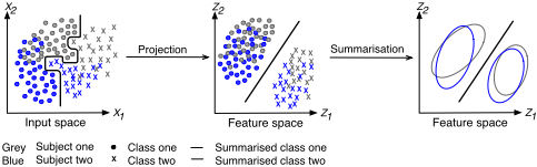
The goal of our work is to efficiently extract features that improve generalisation performance across domains, i.e., features that transfer across domains. We introduce ESRand, an efficient domain generalisation method based on a randomised kernel algorithm, which finds a subspace that minimises the difference between the marginal distributions P(X) of domains, while maintaining the functional relationship P(Y ♣X). In the lower (projected) space, ESRand exploits label information from the training domains and summarises the data by replacing the domains with a set of ellipses and their focal points. While significantly reducing the training time, data summarisation also improves generalisation by eliminating the effect of noisy samples and anomalies.
Through a comprehensive analysis we demonstrate that ESRand has the following desirable properties that distinguish it from previous approaches. Unlike existing domain generalisation approaches that are built based on nonlinear kernels [Blanchard et al., 2011; Muandet et al., 2013; Khosla et al., 2012], ESRand exploits random features in an invariant sub-space to reveal nonlinear patterns in the data. It enables large-scale data processing of computationally expensive machine learning algorithms by significantly reducing the size of the data. Moreover, it outperforms state-of-the-art results on several sensor-based activity recognition benchmark datasets, while being computationally efficient.
2 Background and RelatedWork
ESRand is a domain generalisation method based on randomised kernels, therefore we briefly review these two lines of research in this section.
Domain generalisation: Given several labeled training samples drawn from different sources with biased distributions, domain generalisation assigns class labels to target sets. Fluctuations in the distributions arise in a variety of several applications due to technical, environmental, biological, or other sources of variation. This problem has been addressed in other areas of machine learning such as domain adaptation [Jiang, 2008] and transfer learning [Pan and Yang, 2010]. However, they require the incorporation of target samples or even access to a few of the target labels, while domain generalisation can be performed independent of the target set.
Blanchard et al. [2011] first raised the domain generalisation problem and proposed a kernel-based approach that identifies an appropriate Reproducing Kernel Hilbert Space (RKHS) and optimises a regularised empirical risk over the space. Two projection-based algorithms, Domain-Invariant Component Analysis (DICA) and Unsupervised DICA (UDICA), were then developed by Muandet et al. [2013] to solve the same problem. Extending Kernel PCA (KPCA), DICA and UDICA incorporate the distributional variance across domains to reduce the dissimilarity.
Domain generalisation algorithms also have attracted the computer vision community for object recognition. Khosla et al. [2012] proposed Undoing Dataset Bias (UDB), a multi-task max-margin classifier exploiting dataset-specific biases in feature space. The encoded biases are used to push each dataset's weight to be aligned with the global weights. Xu et al. [2014] proposed an exemplar SVM based method by exploiting the low-rank structure in the source domain. They formulated a new optimisation problem as a nuclear norm-based regulariser that captures the likelihoods of all positive samples. Niu et al. [2015] extended [Xu et al., 2014] and proposed a multiview domain generalisation approach for visual recognition by fusing multiple SVM classifiers. They built upon exemplar SVMs to learn a set of SVM classifiers by using one positive sample and all negative samples in the source domain each time. More recently, Ghifary et al. [2015] proposed a multitask autoencoder that leverages naturally occurring variation in sources as a substitute for the artificially induced corruption, and learns a transformation from the original image into analogs in multiple related domains.
Kernel randomisation: Various nonlinear kernel-machine formulations are used to improve the capacity of learning machines while making learning feasible, e.g., quadratic programming (QP) solvers. In particular, these kernel-based methods rely on the computation of a kernel matrix over all pairs of data points, which limits the scalability of the algorithm on large datasets, and also can limit its effectiveness on high dimensional inputs, given the need to have sufficiently large training samples spanning the variation in the high dimensional space.
To address the scalability problems of kernel-machines, techniques have been proposed that either preprocess the data, e.g., by using dimensionality reduction techniques such as PCA or deep learning [Erfani et al., 2016b], or alleviate the QP problem, e.g., by breaking the problem into smaller pieces, for example by using chunking. A more recent trend explores the use of randomisation, such as linear random projection [Blum, 2006] as a substitute for the computationally expensive step of kernel matrix construction. The work of Rahimi and Recht [2007; 2009] made a breakthrough in this approach. They replicated an Radial Basis Function (RBF) kernel by randomly projecting the data to a lower dimensional space and then used linear algorithms. Random projection avoids the complexity of traditional optimisation methods needed for nonlinear kernels. Recently, randomisation has been applied to other kernel methods, such as dot-product kernels [Kar and Karnick, 2012], and one-class SVM [Erfani et al., 2015; 2016a].
3 ESRand: Elliptical Summary Randomisation
ESRand is a domain generalisation approach based on randomised kernels and elliptical data summarisation, see Figure 1 for an example. The randomised kernel projects the data to a lower-dimensional latent space that minimises the effect of domain bias, while preserving the functional relationship of the data. The Johnson-Lindenstrauss (JL) Lemma provides probabilistic guarantees that the random projection of a dataset to a lower feature space preserves the relative distances between data points. However, the probabilistic nature of the JL-lemma and random projection results in a small number of noisy or outlying data points. To improve the generalisation by further removing noise and outliers in the projected data, we use ellipsoidal summaries to replace the samples. The focal distance between pairs of ellipsoids are then utilised as the dissimilarity measure among domains. In the following, we first formulate the problem and our objective function, and then formally introduce ESRand.
Let Pij denote the distribution of observations over an input space Rn , Xij ⇢ Rn , for a specific setting i 2 ¶1↪ ▷ ▷ ▷ ↪ q♦ which corresponds to a class j 2 ¶1↪ ▷ ▷ ▷ ↪ c♦. For example, Pij can be the distribution of observations collected from a subject (setting) performing a certain activity (class). Therefore, there are two sources of dissimilarity between data distributions in the input space. ESRand transforms the data into a new space Rh to minimise the unwanted dissimilarity introduced by different settings and to preserve/increase the dissimilarity between different classes.
Let D denote the dissimilarity (e.g., focal distance) between two distributions, our objective is to find a transformation φ 2 Rn ⇥ Rh that minimises D(φ(Xj)↪ φ(Y j)), while maximising dissimilarity between classes D(φ(Xj )↪ φ(Y l)), where X and Y are samples from any two subjects. So the objective function has two discordant goals of reducing the distance between some distributions, while increasing the distance between some other distribution, i.e., the functional relationship between dissimilar distributions should be preserved. This leads to the following optimisation problem:
where β and 1 - β show the relative importance of each goal. Note that to yield the best separation, the embedding φ can be different for each activity. The search space of all functions over Rn ⇥Rh is not tractable, so normally the search is conducted over a family of parametric models. In this way, only the parameters of the models have to be found.
3.1 Featurised Kernel Mean Embedding
To learn from data distributions P, we employ a Hilbert space embedding to represent the data distribution as a mean function in a RKHS Hk. The embedding enables efficient computation of the dissimilarities, while maintaining the necessary information of data distributions. Let Hk be an RKHS function f : X ! R, and k be a positive definite function. The kernel mean map of X is defined as
However, since in practice distribution P is unknown, one can use sample data X 2 Rm⇥n drawn from P. Therefore, the sample data is interpreted as the empirical distribution
ˆP = 1m Pmi=1 δxm (·), where δxm (·) is the Dirac delta function at point x 2 X. The empirical kernel mapping (2) is approximated by
In practice, the feature embedding in (2) and (3) may be infinite-dimensional and lack a closed form for some kernels, making it cumbersome for processing large scale datasets. To overcome this limitation, we propose to exploit a lower rank approximation using nonlinear random Fourier features [Rahimi and Recht, 2007], which serves as a good approximation of a nonlinear kernel. For shift-invariant kernels we can exploit Bochner's theorem to generate h-dimensional random features Z 2 Rm⇥h , and for i = 1↪ ▷ ▷ ▷ ↪m
The vectors (w1↪ ▷ ▷ ▷ ↪wh) ⇠ p(w) are sampled from the Fourier transformation, and (b1↪ ▷ ▷ ▷ ↪ bh) ⇠ U(0↪ 2⇡). Then (3) reduces to
3.2 Elliptical Data Summarisation
In the latent space h, our system converts the projected data to elliptical summaries. Then a dissimilarity image of the data is built from a measure of the focal distance between pairs of ellipsoids. Bezdek et al. [2011] defined elliptical summaries for anomaly detection and summarisation of a set of noisy data points. A hyperellipsoidal summary with effective radius ti centred at the sample mean ˜θPi of Zi, with covariance matrix Si is defined as
Remark: (Zi - ˜θPi )T S-1 i (Zi - ˜θPi ) is the Mahalonobis distance fromZi to ˜θPi and S-1 i is the matrix of the hyperellipsoid ei. We use ˜θPi and S-1 i to represent a hyperellipsoidal cluster ei for Zi, whose boundary is defined as
We choose t2 = (χ2 )-1 h (γ) (i.e., the inverse of the chisquared statistic with h-degrees of freedom). This results in an ellipsoid that covers at least 100γ% of the data under the assumption that the data has a Gaussian distribution [Tax and Duin, 2000]. The Gaussian assumption is rarely true for real datasets. However, this threshold is a close approximation for any unimodal distribution. This means that the ellipse for γ selection of h covers the majority points and some of the outlying points are left outside.
The ellipsoid in (7) summarises the data points while removing the effect of outlying samples. We use these ellipsoids instead of the data points as the inputs to the classification techniques. Classification techniques require a distance measure to classify the input objects. This distance measure should capture the differences between the input objects. Three distance measures have been proposed in [Moshtaghi et al., 2011] to measure distances between pairs of ellipsoids. These distances are designed to capture the difference between ellipsoids in terms of eccentricity, location and orientation. Here, we briefly explain the best performing measure called the focal distance.
Let d(ei↪ ej) be the distance between two ellipsoids ei(˜θPi ↪ S-1 i ; ti) and ej(˜θPj ↪S-1 j ; tj). Every plane ellipse e(˜θP↪ S-1 ; t) can be constructed by tracing the curve whose distance from a pair of foci f1 and f2 is a positive constant. The foci always lie on the major axis of the ellipse. If ¶λ-S-1 ↪ λ+S-1♦ are the minimum/maximum eigenvalues of S-1 with corresponding eigenvectors ¶v-↪ v+♦, the foci are
The focal distance between a pair of ellipses ei and ej is an average of a set of four distances. Each component in the average is a distance to one of the focal elements from the other one. Let δ(x↪ y) = kx - yk be the Euclidean distance between vectors in x and y. We have two focal segments with endpoints ¶fi↪1↪ fi↪2♦ and ¶fj↪1↪ fj↪2♦. We compute four distances from δijl and δjil for l 2 ¶1↪ 2♦:
Then the focal distance between ei and ej is computed as:
3.3 ESRand Procedure
To train ESRand, the data collected from c classes of q subjects is first embedded in a subspace using (4) and (5). Then in the feature space, we replace the samples with c ⇥ q ellipsoids using (7), generating one ellipsoid per class of each subject. Instead of solving the optimisation problem in (1), we follow the description in Section 4 and generate a projection φ 2 Rn⇥h that obtains dissimilarities satisfying the conditions in (1). The test procedure is similar to the training procedure, projecting the test data to the feature space by applying φ, and summarising the samples with ellipsoids. When ESRand is used in conjunction with k-NN, the test ellipsoids are classified w.r.t. their focal distance to the closest training ellipsoids; and when used with SVM the focal points and their associated labels are the input to the algorithm.
4 Theoretical Justification
Random projection is a dimensionality reduction method that has been widely adopted in machine learning [Rahimi and Recht, 2007; Oymak and Tropp, 2015]. The first result, known as the JL-Lemma, states that for a given a set of points in a high-dimensional space, there is a projection into a lowerdimensional random subspace that preserves the functional relationship of the data (e.g., the inter-point distances and angles with high probability). Here, the most important implication is that if we have data that is separated by some small margin, then a random linear separator would probably be a weak learner with error less than 1◁2. Therefore, we can combine kernel functions with the JL-Lemma to note that if a learning problem has a large margin under the kernel k(·↪ x), then a random linear projection of the Hilbert space down to a sub-space approximately preserves linear separability.
While the random projector should preserve geometric features of the set, we do not want to map a point in the set to the origin. To ensure this, we refer to the results in [Oymak and Tropp, 2015]: the success probability and stability of a random projection for a given set depends on the embedding dimension that can be quantified through universality theorems in high-dimensional stochastic geometry.
Theorem 1 A Universality Law for the Embedding Dimension. Given the n ⇥ h random projector φ with the parameters p > 4, ⌫ ≥ 1, % 2 (0↪ 1), and " 2 (0↪ 1), there is a number N := N(p↪ ⌫↪ %↪ ") for which the following statement holds. Suppose that the ambient dimension n ≥ N; E is a nonempty, compact subset of Rn that does not contain the origin; the statistical dimension of E is proportional to the ambient dimension: %n ✓(E) n. Then h ≥ (1 + ")✓(E) implies P¶0 ◁2 φ(E)♦ ≥ 1 - Cpn1- p4 . Furthermore, if ✓(E) is spherically convex, then h (1 - ")✓(E) implies P¶0 2 φ(E)♦ ≥ 1 - Cpn1- p4 .
This theorem ensures that the random projection succeeds for a spherically convex set E when the embedding dimension h exceeds the statistical dimension ✓(E) where 0 < ✓(E) n and can be computed through ✓(E) = E[(max b2✓ g▷b)2+]↪ g 2
N(0↪ I). To simplify this, let ⌦ be a closed, spherically convex set in Rn ; and the entries of the random projector φ : Rn ! Rh be small, constant, partly non-zero, standardised, independent, and symmetric, with a modest amount of regularity. For this class of random projectors, it has been proved that
where o(n) depends only on the regularity of the random variables. Therefore, over the mentioned class of random projectors, the phase transition in the embedding dimension is universal, provided that ⌦ is not too much smaller than the original dimension n. In the other words, there is a substantial class of random projectors for which the phase transition in the embedding dimension is universal. Moreover, it is important to quantify the stability properties of randomised dimension reduction. The stability of the random projector on a compact, convex set E in Rh can be quantified using the universality theorem for the restricted minimum singular value.
Theorem 2 Universality for the Restricted Minimum Singular Value. Given the random projector φ : Rn ! Rh with the fixed parameters p, ⌫, % 2 (0↪ 1), λ 2 (0↪ 1), and ✏ 2 (0↪ 1), there is a number N := N(p↪ ⌫↪ %↪ ✏) for which the following statement holds. Suppose that the ambient dimension n ≥ N; E is a nonempty, compact subset of the unit ball Bn in Rn ; the embedding dimension d is in the range λn h n6◁5 ; the h-excess width of E is not too small: "h(E) ≥ %ph. Then P¶σmin(φ;E) ≥ (1-✏)("h(E))+♦ ≥ 1-Cpn1-p◁4 ▷ Furthermore, if E is convex, then P¶σmin(φ; E) (1+✏)("h(E))+♦ ≥ 1-Cpn1-p◁4 where the constant Cp depends only on the parameter p in the random matrix model.
For any random projector, Theorem II proves that the distance of the random projection from the origin cannot be much smaller than the h-excess width "h(E). Similarly, when E is convex, the distance of the random projection from the origin cannot be much larger than the h-excess width. The excess width "h(E) is not much smaller than the embedding dimension ph. Correspondingly, the random projection is stable and far from the origin, i.e., the embedding succeeds, if the restricted minimum singular value is large enough. Detailed proofs can be found in [Oymak and Tropp, 2015].
5 Empirical Analysis
In this section, we illustrate the effectiveness of ESRand via a visualisation of a toy dataset. Furthermore, we compare the performance and efficiency of the proposed algorithm with state-of-the-art algorithms through classification tasks on multiple benchmark datasets.
Datasets: The experiments are conducted on four real life datasets from the UCI Machine Learning Repository: (i) Daily and Sport Activity (DSA), (ii) Heterogeneity Activity Recognition (HAR), (iii) Opportunity Activity Recognition (OAR), (iv) PAMAP2 Physical Activity Monitoring, with the number of 19, 6, 5, 13 activities collected from 8, 9, 4, 8 subjects, respectively 1 . All the records in each dataset are normalised between [0,1].
Baselines: To evaluate the performance and efficiency of ESRand, we compare it with the following baseline methods: (i) KPCA, (ii) DICA and UDICA: kernel-based optimisation algorithms that learn an invariant transformation to minimise the dissimilarity across domains, (iii) AE (Autoencoder) [Bengio et al., 2007]: a basic autoencoder trained by stochastic gradient descent, (iv) CAE (Contractive Autoencoder) [Rifai et al., 2011]: an autoencoder with an additional penalty, the Frobenius norm of the Jacobian matrix of the encoder activations with respect to the input, to yield robust features on the activation layer, (v) k-NN: k Nearest Neighbour, we use k = 1, (vi) SVM: Support Vector Machine with RBF kernel, (vii) UDB: a max-margin SVM-based framework for reducing dataset bias, (viii) LRE-SVM [Xu et al., 2014]: a non-linear exemplar-SVMs model with a nuclear norm regularisation to impose a low-rank likelihood matrix.
The hyper-parameters of all the algorithms are adjusted using grid search based on their best performance on a validation set. Algorithms i - iv are used for feature extraction. For classification purposes, the learnt features from these algorithms are used with k-NN and multi-class SVM with a linear kernel l-SVM. Since the focus of the experiment is to evaluate the effectiveness of feature extraction methods, we utilise simple classification algorithms, otherwise more advanced approaches can be employed. For algorithms v - viii no feature extraction has been conducted, and the algorithms have been applied directly on the (normalised) raw datasets.
1 DSA, HAR and PAMAP2 are large datasets including millions of samples. We used a subset of these datasets. For DSA and PAMAP2 the first 1000 samples of each activity from each user were used, and for HAR the first 2000 samples were used.
Metric: We use the Receiver Operating Characteristic (ROC) curve and the corresponding Area Under the Curve (AUC) to measure the performance of all the methods. The reported AUC values of each algorithm are the average accuracies of leave-one-domain-out test (domain), i.e., taking one domain as the test set and the remaining domains as the training set. The reported training times are in seconds, and the stated AUC values and training times are the average of 20 folds for each experiment. For SVM based methods LIBSVM was used.
5.1 Visualisation
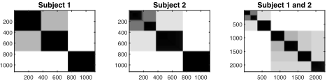
To demonstrate the impact of ESRand, we used a toy dataset, a subset of the DSA dataset including the first 375 samples from three activities of two subjects, and a visualisation tool called improved Visual Assessment of cluster Tendency (iVAT) [Wang et al., 2010]. iVAT helps to visualise the possible number of clusters in a set of objects, by reordering the dissimilarity matrix of the objects so that it can display any clusters as dark blocks along the diagonal of the image.
Figure 2, from the left, shows the images of the raw toy dataset from subject 1, subject 2, and their combination, respectively. The first two images show three dark blocks indicating three activities of each subject. When combining the two datasets, it is expected that similar activities of the two subjects should overlap, however, the image shows six distinct blocks due to bias in the domains' distribution.
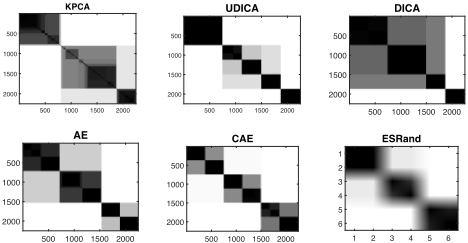
Figure 3 compares the impact of ESRand with i - iv projection baselines on the toy dataset. Among all, only the autoencoder based approaches (AE and CAE) and ESRand manage to reduce the six clusters, in the combined dataset, to the three main clusters. It is noteworthy that unlike all the other feature extraction methods, algorithms i - iv, ESRand summarises the dataset, reducing the total number of sample points from M = 2250, i.e., M = mqc the number of samples⇥subjects⇥activities, in this example to 6 (qc). This major reduction in data size is expected to alleviate classification time significantly. In the following, we explore whether these feature extraction yields better classification accuracy, and how data summarisation accelerates classification time.
| k - NN | l-SVM | |||||||||||||
|---|---|---|---|---|---|---|---|---|---|---|---|---|---|---|
| Dataset | KPCA | DICA | AE | CAE | ESRand | KPCA | DICA | AE | CAE | ESRand | k-NN | SVM | UDB | LRE |
| DSA | 87 ◦ 6 | 88 ◦ 5 | 90 ◦ 3 | 95◦ 3 | 95◦ 1 | 85 ◦ 9 | 87 ◦ 4 | 92 ◦ 2 | 94 ◦ 1 | 96◦ 0 | 88 ◦ 6 | 86 ◦ 6 | 89◦3 | 92 ◦ 4 |
| HAR | 61 ◦ 10 | 68 ◦ 9 | 76 ◦ 6 | 84 ◦ 2 | 87◦ 2 | 60 ◦ 8 | 63 ◦ 6 | 77 ◦ 3 | 83 ◦ 1 | 86◦ 1 | 65 ◦ 8 | 74 ◦ 11 | 76 ◦ 4 | 80 ◦ 3 |
| OAR | 72 ◦ 5 | 73 ◦ 3 | 79 ◦ 5 | 85 ◦ 2 | 89◦ 1 | 73 ◦ 8 | 74 ◦ 5 | 76 ◦ 4 | 86 ◦ 2 | 88◦ 1 | 72 ◦ 4 | 71 ◦ 7 | 77 ◦ 5 | 79 ◦ 6 |
| PAMAP2 | 81 ◦ 4 | 81 ◦ 3 | 91 ◦ 2 | 95 ◦ 2 | 97◦ 0 | 79 ◦ 3 | 82 ◦ 5 | 91 ◦ 1 | 97◦ 2 | 97◦ 1 | 79 ◦ 4 | 83 ◦ 3 | 85 ◦ 3 | 89 ◦ 2 |
| Avg. | 75 ◦ 7 | 78 ◦ 5 | 84 ◦ 4 | 90 ◦ 2 | 92◦ 1 | 74 ◦ 7 | 77 ◦ 5 | 84 ◦ 2 | 90 ◦ 2 | 92◦ 2 | 76 ◦ 6 | 79 ◦ 7 | 82 ◦ 4 | 85 ◦ 4 |
5.2 Accuracy Evaluation
Table 1 compares the accuracy values of the baselines against ESRand. The reported values are the percentage of accuracy ◦ the standard deviation. Since the accuracy results of UDICA and DICA are comparable on these dataset, only the results of DICA have been included in the table. On average, the algorithm with the best performance on these datasets is ESRand with an average accuracy of 92%. The closest results are from CAE, with 90% accuracy. To statistically assess the significance of the performance between the two algorithms, we use the Wilcoxon signed-rank test. The test returns a p-value 0▷0312 rejecting the null hypothesis for the accuracy with a level of significance of ↵ = 0▷05. This result implies a significant improvement of ESRand over the CAE. Although the added penalty term to CAE enhances the feature learning of the basic autoenoder AE, it does not yield comparable accuracy to ESRand. This indicates that enhancing the feature learning strategy can provide better discriminative features with respect to unseen samples. Observing the standard divisions from Table 1, ESRand also yields more consistent results with the lowest standard deviation on average.
A possible explanation for the effectiveness of ESRand can relate to the dimensionality of the manifold in feature space where samples concentrate. We hypothesise that if features concentrate near a low dimensional sub-manifold, then the algorithm has found invariant features and will generalise well. Moreover, the data summarisation eliminates noisy records and outliers, which can give a boost to the generalisation.
5.3 Efficiency Evaluation
A desirable property of ESRand is that it summarises datasets, substantially reducing the number of samples as well as the number of features. To study this impact we compare the training time of ESRand with CAE, which has the second best accuracy and linear time complexity of O(Mn). In this experiment we used DSA and PAMPA2, the datasets with a large number of activities. The first comparison is between ESRand and CAE, which shows the training time of these two algorithms without including the classification time. As can be seen in Figure 4, the training time of ESRand grows linearly with a much more gentle slope than CAE.
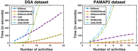
Comparing the training time of l-SVM on the output of these two algorithms (i.e., l-SVM(ESRand) and l-SVM(CAE)) reveals the advantage of ESRand's data summarisation. The training time of l-SVM on the summarised output of ESRand remains fairly low, while on CAE it soars. The total training time of ESRand+l-SVM remains significantly lower than CAE+l-SVM. With large datasets, searching for the pair of variables that maximise class separation is a computationally expensive procedure. The computational complexity of most common algorithms such as k-NN and SVM is quadratic in the total number of records M. As discussed earlier, ESRand reduces the size of training data to q ⇥ c. More specifically, the time complexity of ESRand is computed as O(Mn) + O(Mh2 ), and when h ⌧ n then the complexity reduces to O(Mn), and the size of ESRand's output reduces from RM⇥n to Rqc⇥h .
6 Conclusion
We have presented ESRand, an efficient domain generalisation method that aims to reduce distribution bias in multi-domain learning. ESRand incorporates a simple but effective random projection with an elliptical data summarisation to overcome distribution variance across domains. Our analysis on several benchmark activity recognition datasets reveals that ESRand successfully learns domain-invariant features, yielding stateof-the-art performance from unseen target domains. Moreover, ESRand enables large-scale data processing by significantly reducing the size of data, in both the dimensionality and the number of samples.
@inproceedings{ijcai2016p209,
  title     = {Robust Domain Generalisation by Enforcing Distribution Invariance},
  author    = {Erfani, Sarah M. and Baktashmotlagh, Mahsa and Moshtaghi, Masud and Nguyen, Vinh and Leckie, Christopher and Bailey, James and Ramamohanarao, Kotagiri},
  booktitle = {Proceedings of the Twenty-Fifth International Joint Conference on
               Artificial Intelligence, {IJCAI-16}},
  publisher = {AAAI Press / International Joint Conferences on Artificial Intelligence},
  editor    = {Subbarao Kambhampati},
  pages     = {1455--1460},
  year      = {2016},
  month     = {7},
  url       = {https://ijcai.org/proceedings/2016/209},
}
TY - CPAPER TI - Robust Domain Generalisation by Enforcing Distribution Invariance AU - Erfani, Sarah M. AU - Baktashmotlagh, Mahsa AU - Moshtaghi, Masud AU - Nguyen, Vinh AU - Leckie, Christopher AU - Bailey, James AU - Ramamohanarao, Kotagiri T2 - Proceedings of the Twenty-Fifth International Joint Conference on Artificial Intelligence, IJCAI-16 PB - AAAI Press / International Joint Conferences on Artificial Intelligence PY - 2016 SP - 1455 EP - 1460 UR - https://ijcai.org/proceedings/2016/209 ER -Copied
Machine-readable versions of this paper, for tools and AI agents:





