Tight Policy Regret Bounds for Improving and Decaying Bandits

1 Introduction

In the well-studied multi-armed bandit setting, a decision maker is faced with the problem of choosing which arm to play over a sequence of trials. Each time the decision maker pulls an arm, he receives a reward, and his goal is to minimize some notion of regret. The majority of previous studies consider the so-called external regret as the objective. External regret is the difference between the total reward collected by an online algorithm and the maximum reward that could have been collected by pulling a single arm on the same sequence of rewards as the one generated by the algorithm. Past solutions to this problem can be divided into two main categories: first, solutions that rely on statistical assumptions about the underlying reward process (see for instance[Robbins, 1985; Gittins et al., 2011; Auer et al., 2002]); and second, solutions for the setting where an adversary, who is capable of reacting to the choices of the decision maker, determines the sequence of rewards (see e.g. [Auer et al., 2002]).

Aaron Roth

University of Pennsylvania aaroth@cis.upenn.edu

Our goal in this work is to minimize a stronger notion of regret, namely policy regret, in a setting where the reward from each arm changes monotonically 1 every time the decision maker pulls that arm. More precisely, in the model we propose, there exist n arms, each with a reward curve that is unknown to the decision maker. Every time the decision maker pulls an arm, the corresponding reward of that arm monotonically changes according to its underlying reward curve.

Unlike traditional statistical approaches, we do not make probabilistic assumptions on the behavior of the arms; and unlike traditional adversarial approaches, we do not assume a fixed sequence of payoffs against which we measure our regret. In particular, under our assumptions the algorithm itself is actually generating the sequence of payoffs via its decisions. The right notion of regret is thus not comparing to the best single arm in hindsight on the sequence generated (external regret), but to the best sequence that could have been generated - that is, to the optimal policy that knows the reward functions. This stronger notion is what is called policy regret in the literature [Arora et al., 2012]. The following simple example further illustrates the difference between policy and external regret.

Example 1 Consider a setting in which there are two arms and time horizon T ≫ 10. Arm 1 returns a reward of iT when pulled for the ith time, and arm 2 always returns a reward of 0.1. Consider the algorithm that always pulls arm 2. The external regret of this algorithm is zero because at every time step, it pulls the arm that would give it the largest reward on that time step. But the policy regret of this algorithm grows linearly with T, as the best policy in hindsight indeed pulls arm 1 at every time step. 2

We are motivated by settings in which the available actions correspond to the assignment of a sequence of relatively homogeneous tasks to one of a finite set of workers, as is often the case in crowdsourcing systems (see for example [TranThanh et al., 2014; Heidari and Kearns, 2013]). In such settings, it is reasonable to expect that workers' performance may improve or decay with repeated trials, depending on the nature of the task. For example, tasks that are unfamiliar and challenging (such as segmenting brain images into individual neurons [Seung, 2015]) may require a training period during which performance gradually improves. In contrast, in a task primarily requiring only human perception (such as the transcription of license plates in images [Barowy et al., 2012; Du et al., 2013]), subjects may immediately be able to perform the task at a high level, but its tedious and taxing nature may lead to performance decay with increased workload. In both cases, different subjects may have different rates of improvement or decay.

1 See [Slivkins, 2011] for other motivating examples and a different formalization of monotone bandits.

2 It is easy to adapt this example to show that specific algorithms with no external regret, such as EXP3, will indeed fail to have small policy regret.

The rest of this paper is organized as follows: In Section 2, we introduce the model. In Section 3, we study the case of increasing and concave reward functions and present an optimal online algorithm whose policy regret depends on a parameter we call ⌧. This parameter quantifies the time required to distinguish the optimal arm from the others, and we prove the dependence is necessary. We prove that the policy regret of this algorithm is sublinear and further illustrate the range of behaviors of ⌧ and the performance of the algorithm via simulations. Finally, in Section 4 we investigate the case of decreasing rewards and present a provably optimal algorithm whose policy regret is constant and upper bounded by the number of arms.

1.1 RelatedWork

As discussed in [Arora et al., 2012], the notion of external regret fails to capture the actual regret of an online algorithm compared to the optimal sequence of actions it could have taken when the adversary is adaptive. Policy regret is defined to address this counterfactual setting. The authors show in [Arora et al., 2012] that if the adaptive adversary has bounded memory, then a variant of traditional online learning algorithms can still guarantee no policy regret. In our work, the rewards depend on all the actions taken so far and as the result our model is not captured by the bounded memory setting.

While our model is not captured by any of the previous papers in the bandit literature, the following papers are conceptually related. [Tekin and Liu, 2012] study a setting in which the reward from each arm is modeled as a finite-state Markov chain. Authors consider two cases: rested and restless arms. In the rested case, the state of each underlying Markov chain remains frozen unless the corresponding arm is played. While in our setting the arms are indeed rested, the reward process we study cannot be modeled by a finite-state Markov chain (see also [Neu et al., 2014]). [Gabillon et al., 2013] studies the problem of picking a subset of arms at each step in a setting where the reward is a submodular function of the chosen subset. [Streeter et al., 2009] studies the problem of assigning items to K positions such that a submodular utility function is maximized. Finally, our model is somewhat related to the line of research on best arm identification, however, previous studies on this topic mainly rely on stochastic assumptions on the rewards (see for example [Audibert and Bubeck, 2010],[Chandrasekaran and Karp, 2012]), and they do not apply to our setting.

There is much work in the psychology literature studying the human learning process on cognitive tasks (see e.g. [Atkinson et al., 1965; Mangal, 2009]), but to our knowledge ours is the first to model it in a bandits setting. There are however, a limited number of papers addressing relevant questions from a heuristic or empirical viewpoint (see [Basu and Christensen, 2013; Singla et al., 2013]).

2 Model and Preliminaries

The decision maker has access to n arms denoted ¶1↪ 2↪ ▷▷▷↪ n♦. At each time step t (t = 1↪ 2↪ ▷▷▷↪ T ) he has to decide which arm to pull. Every time the decision maker pulls an arm, he collects a reward and his goal is to pull the arms in such a way that his policy regret (to be formally defined shortly) is minimized. We assume the decision maker knows the time horizon T in advance.

We model the reward process of the arms as follows: Each arm k has a fixed underlying reward function denoted by fk(▷). When the decision maker pulls arm k for the mth time (m ≥ 1), he receives an instantaneous reward equal to fk(m). The cumulative reward from pulling arm k for m times is denoted by Fk(m) and is equal to fk(1) + fk(2) + ▷▷▷ + fk(m). We assume that all the reward functions are bounded from below by 0 and from above by 1 3 .

A deterministic policy ⇡ of length T is a sequence of mappings h⇡1↪ ⇡2↪ ▷▷▷↪ ⇡T i from the histories to the arms. That is,

prescribes the arm that must be pulled at step t given the history of actions and rewards observed so far. Given the reward functions f1(▷)↪ ▷▷▷↪ fn(▷) and a deterministic policy ⇡, the arm that the policy picks at each time step t is deterministic and is denoted by it. Let btk (⇡) be the instantaneous reward of arm k under policy ⇡. More precisely, suppose the decision maker has followed policy ⇡ up until time (t - 1). btk (⇡) denotes the reward of playing arm k at time t. (As it is usually clear from the context what policy we are referring to, for simplicity we drop ⇡ in our notation.) Note the difference between fk(t) and btk : unlike fk(t), btk depends on the history of actions taken so far, in particular, the number of times arm k has been pulled before time t by policy ⇡. We denote by r(⇡) the total reward that a policy ⇡ collects, so r(⇡) = PTt=1 btit . Note that the total reward of a policy only depends on the number of times each arm is pulled and not the order.

Given the reward functions f1(▷)↪ ▷▷▷↪ fn(▷) and T , let OPT be the policy that maximizes the total reward. In the online setting, the decision maker does not know the reward functions in advance and seeks to design a (possibly randomized) algorithm A so that the total reward he collects is as close as possible to that of OPT. In other words, the decision maker's goal is to minimize his policy regret which is defined as r(OPT) - Er(A). We say that an online algorithm A has sublinear policy regret if

3 It is easy to see that without this assumption no algorithm can guarantee sublinear policy regret.

3 Increasing Reward Functions

3.1 The Offline Setting

We first show that when the reward curves are all increasing, there exists a single best arm that the optimal policy must repeatedly pull. Despite this fact, merely having the guarantee of no external regret would not be sufficient to guarantee no policy regret here (see Example 1).

Proposition 1 Suppose for all 1  k  n, fk(▷) is increasing. Then there exists an arm k⇤T such that the optimal offline policy OPT consists of pulling k⇤T for all T trials.

Proof Assume OPT pulls arm k, Tk times (so Pni=1 Ti = T ). Suppose there exist arms i↪ j for which Ti↪ Tj > 0. We claim that fi(0) = fj(0) = fi(Ti) = fj(Tj). In other words, fi↪ fj are both flat and identical. If this holds, the policy OPT remains optimal if we replace every occurrence of i in it with j. Repeating this for any two arms i0 ↪ j 0 with Ti0 ↪ Tj 0 > 0, we see that OPT consists of pulling a single arm T times.

To prove the above claim, we first note that since all the fks are increasing, it must be that fi(Ti) ≥ fj(Tj). Otherwise one could collect a reward larger than OPT by never pulling arm i and instead pulling arm j for Tj + Ti times. But this is a contradiction with optimality of OPT. Similarly fi(Ti)  fj(Tj) and therefore, we can conclude fi(Ti) = fj(Tj). Next we observe that fi(0) ≥ fj(Tj). Otherwise, given that fi(Ti)  fj(Tj), one could collect a reward larger than OPT by never pulling arm i and instead pulling arm j for Ti additional times. Combining this with the previous equality, we can conclude that fi(Ti) ≥ fi(0) ≥ fj(Tj) = fi(Ti) and therefore, fi(0) = fi(Ti). Similar argument holds for j as well. Therefore, fi(Ti) = fi(0) = fj(Tj) = fj(0). This proves our claim and finishes the proof.

3.2 The Online Setting

In addition to being increasing and bounded, we assume the learning curves satisfy decreasing marginal returns (see Section 5 for a discussion of why this assumption is needed). More precisely, for any arm k we assume

If we think of the reward curves as continuous functions, the concavity of fk would give us decreasing marginal returns. Therefore we slightly abuse the terminology and refer to this property as "concavity". We emphasize that the concavity assumption is very natural and common in the context of human learning (see for example [Son and Sethi, 2006]) and in particular, concave learning curves have been shown to arise in various laboratory environments (see for example [Jovanovic and Nyarko, 1995; Anderson and Schooler, 1991]).

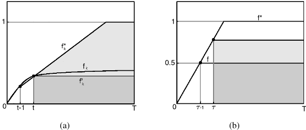
For the case where the reward functions are all increasing, bounded and concave, we introduce an online algorithm whose policy regret bound, as we shall prove, is sublinear and optimal. Our algorithm is motivated by the following observation: Suppose we initially pull arm k, t times and observe fk(1)↪ fk(2)↪ ▷▷▷↪ fk(t). After this, given that fk is increasing, we can be sure that for any t < s  T, fk(s) ≥ fk(t). In other words, the additional reward that can be collected from arm k in the remaining (T - t) steps is minimized if fk flattens at t. We define the pessimistic estimate of the total reward from arm k (denoted by qtk (T )) to be equal to the total reward of a function f 0k that is identical to fk up to t, and then flattens out 4 (see Figure 1 (a)).

In addition to the above lower bound, concavity yields an upper bound on future payoffs. The additional reward that can be collected from arm k in the remaining (T - t) steps is maximized if the function continues to grow linearly with rate (fk(t) - fk(t - 1)). We define the optimistic estimate of the total reward from arm k ( denoted by ptk (T )) to be equal to the total reward of a function f 00 k that is identical to fk up to t, and then continues to grow linearly with rate (fk(t) - fk(t - 1)) until it hits 1 5 (See Figure 1 (a)).

Since all the reward curves are increasing, by Proposition 1 we know that there exists a single best arm that is repeatedly pulled by the optimal policy. Therefore we seek to detect this arm. Our algorithm operates as follows: it maintains a set of candidate arms in which the best arm is guaranteed to lie. At each round, it pulls all the arms in the candidate set exactly once, and updates both optimistic and pessimistic estimates of the reward from these arms. If at some round the optimistic estimate of an arm k is less than or equal to the pessimistic estimate of another arm in the candidate set, then we are sure that k can not be the optimal arm, and therefore the algorithm eliminates it from the candidate set. See algorithm 1 for the details. We refer to this algorithm by A1.

For the coming theorem, we make use of a quantity that captures the time required to distinguish the optimal arm from the others. More precisely, we define ⌧(T) = maxk ⌧k(T) where

and k⇤T is the optimal arm for the time horizon T . Thus ⌧k(T ) specifies the smallest number of times we need to pull both arm k and k⇤T so that the optimistic estimate of the total reward from arm k falls behind the pessimistic estimate of the total reward from arm k⇤T .

We now prove that the policy regret of A1 is bounded by n⌧(T), and show that this is optimal. Eventually in Theorem 2 we shall prove the regret of A1 is in fact sublinear.

Theorem 1 Suppose for all 1  k  n, fk(▷) is concave, increasing, bounded from below by 0 and from above by 1. Then 6

Furthermore, the policy regret bound of A1 is optimal: there exists a family of examples consisting of bounded, increasing and concave reward functions for which no algorithm can be guaranteed to have a policy regret bound of o(n⌧(T)).

Proof Observe that A1 detects the optimal arm after at most ⌧(T) phases. This is simply because a suboptimal arm k is

6 One can easily see that with the exact same logic as the one in the proof of Theorem 1, we can get a slightly better upper bound of Pnk=1 ⌧k(T) on the regret, but to simplify the statement of the theorem and its proof, we work with the worst case upper bound of n⌧ (T ).

Algorithm 1 The online algorithm for concave and increasing

reward functions (A1) t = 0; % t is the index of the current phase. S = ¶1↪ ▷▷▷↪ n♦; % S is the set of remaining candidate arms. Pull every arm exactly once. repeat t = t +1; % Start a new phase for each i 2 S do Pull arm i once. pti (T) = Fi(t) + PTs=t+1 min¶1↪ fi(t) + (f(t) - f(t -1)) (s - t)♦; % Update the optimistic estimate. qt i (T) = Fi(t) + fi(t)(T - t); % Update the pessimistic estimate. end for for i 6= j 2 S do if qt j (T) > pti (T) % i.e. there exists an arm whose total reward is guaranteed to be larger than that of arm i then S = S ∩ ¶i♦. end if end for until only one arm remains in S or time runs out. For the remaining steps (if any), pull the only arm left in S.

removed from S by phase ⌧k(T). In addition, note that arm k⇤T can never be removed from S due to its optimality. Therefore, we can conclude that the number of times when A1 pulls suboptimals arm is at most n⌧(T). Combining this with the fact that the reward per step is upper-bounded by 1 yields the desired inequality.

For the lower bound, fix a constant ⌧ < T, and consider n arms that all have linear reward curves with identical slope of 1 2(⌧-1) , until they reach payoff 0▷5 at time (⌧ - 1). Then (n-1) of the curves stay at 0▷5 forever, whereas one of them selected at random continues to 1 (see Figure 1 (b)). It is easy to see that for any T > ⌧, ⌧(T) = ⌧. Using Yao's min-max principle [Yao, 1977], we lower-bound the regret of any deterministic algorithm on the above randomized setting. Let us define the number of arms an algorithm verifies to be equal to the number of arms that it pulls at least ⌧ times (note that this is well-defined for any deterministic algorithm). It is easy to see that in this example, no algorithm can find the optimal arm with high probability by verifying o(n) arms. To see this, first note that in order to see whether an arm is optimal, the algorithm has to pull it at least ⌧ times. Assume, without loss of generality, that the first arm that the algorithm verifies is arm 1, the second one is arm 2, and so on. Since the index of the optimal arm is chosen uniformly at random, the expected number of arms the algorithm must verify before finding the optimal arm is equal to Pn-1 i=0 in = 1n n(n-1) 2 = (n-1) 2 . Every time the algorithm verifies a sub-optimal arm, it fails to collect at least 0▷5⌧ units of reward from the optimal arm, and instead obtains a reward on average equal to 0▷25⌧ . As a result the policy regret of the algorithm is lower bounded by ⌧(n-2) 2 .

Next we show that the policy regret of Algorithm 1 is in fact sublinear for any choice of bounded, concave and increasing reward functions f1(▷)↪ ▷▷▷↪ fn(▷). The following notation will be useful in our argument: we denote the asymptote of fi(▷) by ai, i.e.

Note that since fk(▷) is increasing and bounded, the asymptote exists and is finite. Also for any arm i limT!1 Fi(T) T = ai. We define a⇤ to be max1in ai, and

Theorem 2 For any set of bounded, concave, and increasing reward function f1(▷)↪ ▷▷▷↪ fn(▷), the policy regret of A1 is sublinear.

Here is the outline of the proof: We start by observing that for large values of T, the optimal arm must have the largest asymptote among other arms (note that we don't assume there is only one arm with maximum asymptote). Therefore a suboptimal arm i can be of one of the following two types:

1. The asymptote of arm i is smaller than that of the optimal arm; For this case, we show that A1 dismisses arm

i from its candidate set within o(T) phases. As a result the regret from pulling arm i cannot not large.

1. The asymptote of arm i is equal to that of the optimal arm; For this case, we show that while A1 may fail to determine the suboptimality of arm i quickly, since the asymptote of i is as large as the optimal arm, pulling it does not add much to the policy regret of A1.

Proof Observe that limT!1ak⇤T = a⇤ ; in other words, if T is sufficiently large, then k⇤T 2 argmax1in ai. Throughout, we assume T is large enough so that the latter holds.

Let W = argmaxk ak. We start by showing that if i 62 W (i.e. ai < a⇤ ), then A1 removes arm i from its candidate set within o(T ) phases.

Proof Suppose that the statement of the lemma does not hold and limT!1 ⌧i(T) T 6= 0. This means that for any unbounded and increasing sequence ¶γT♦1T=1 for which limT!1 γT T = 0, there exists an infinite subsequence of T's such that qγT k⇤ (T) < pγT i (T). Expanding this, we have 7

The above is equivalent to

Therefore combined we have:

Now note that if T (and as a result γT ) is large enough, then Fk⇤T (γT ) ≥ Fi(γT ) and fk⇤T (γT ) - fi(γT ) ≥ ak⇤T -ai 2 = a⇤-ai 2 . Let C = a⇤-ai 2 (recall that due to our assumption about arm i, C > 0). Therefore from (1) we obtain that C(T - γT ) < ∆i(γT ) T 2 2 and as a result

where the last inequality follows from the fact that limT!1 γT T = 0. So we have

7 To simplify the notation in this equation we drop the subscript T . Also by δi we mean ∆i(γ).

Next, one can easily verify that limT!1∆i(γT )T = 0. To see this note that

where the last inequality follows from the fact that ¶γT♦1T=1 is positive, increasing and unbounded. This combined with (2) yields C  0, which is a contradiction.

Second we show that if i 2 W (i.e. ai = a⇤ ), while A1 may fail to detect the suboptimality of arm i quickly, pulling arm i does not add much to the policy regret of A1.

Using Lemma 1, we can conclude that for any arm i 62 W our algorithm can distinguish i from k⇤ within o(T) phases. In other words, after a prefix of at most o(T) many phases, A1 eliminates every arm i 62 W.

Lemma 2 Let Ti denote the number of times A1 pulls arm i 2W. Then

Proof If i 2 W gets eliminated within o(T ) phases, it can not cause the algorithm to suffer from a linear policy regret. Now consider a subset W 0 of W consisting of any suboptimal arm i for which it takes ⇥(T) steps for the algorithm to eliminate

i. Given that the arms not in W 0 can all be detected in T 0 = o(T) time steps, we have that T - Pi2S0 Ti = T 0 = o(T). Let w 2 W 0 be the arm for which Fi(Ti) Ti is the smallest. We

have

That is,

It only remains to show that

But this is certainly true as limT!1 Fk⇤T (T ) T = limTw!1 Fw(Tw) Tw = a⇤ . Combining (3), (4), we have the desired result.

Combining Lemma 1 and 2 we obtain the sublinearity of the policy regret for A1.

Finally, we remark that if the decision maker only gets to observe a corrupted version of the rewards and the corruption is bounded by some ✏ > 0, then A1 is guaranteed to have a total reward at least equal to r(OPT)-n⌧ ✏ (T). ⌧ ✏ (T) is the corrupted version of ⌧(T) in which the optimistic and pessimistic estimate from an arm are computed by taking the presence of noise into account 8 .

3.3 Simulations

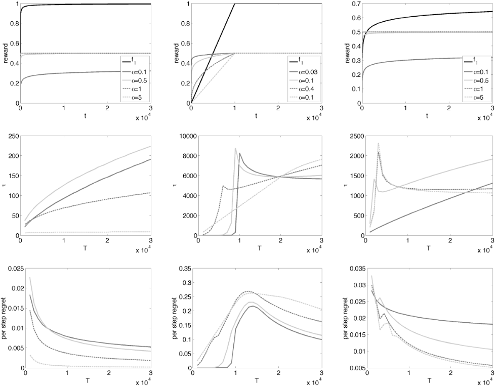
So far we have established two upper bounds on the regret of A1: in Theorem 1 we gave an upper bound of n⌧(T), and in Theorem 2 we showed that the regret of is always sublinear. In this section we empirically investigate the performance of A1 on several illustrative reward curves, and observe that ⌧(T) (and the regret of our algorithm) are typically significantly sublinear in T .

Throughout, for simplicity we set n to 2 and consider two arms 1↪ 2 where the asymptote of f1 is 1 and that of f2 is 0.5. In Figure 2, we report the value of regret and ⌧ versus T = 500↪ ▷▷▷↪ 30000 for three different sets of examples.

In the first column of Figure 2, f1(t) = 1 - t-0▷5 and f2(t) = 0▷5 - 0▷5t-↵ where ↵ = 0▷1↪ 0▷5↪ 1↪ 5. Each of these values corresponds to a different rate of increase for f2. The larger ↵ is, the faster f2 converges to its asymptote. In this example for all values of ↵, ⌧ increases slowly (sub-linearly) with T and as a result regret consistently decreases with T. The reason for the slow growth of ⌧ is that f1 converges to its asymptote very quickly; in addition, the rate with which f2 increases, approaches 0 fast. This enables the algorithm to find and dismiss the suboptimal arms early on.

In the second column, f1(t) = min¶1↪ t 30000 ♦ and f2(t) = min¶0▷5↪ 0▷5( t 30000 )↵♦ where ↵ = 0▷03↪ 0▷1↪ 0▷4↪ 1. The smaller ↵ is, the faster f2 converges to its asymptote. Here when ⌧ increases linearly or faster with T , the regret increases as well. Note that this does not contradict Theorem 2 as the theorem holds for large enough values of T only. Notice that for ↵ = 0▷03↪ 0▷1↪ 0▷4, ⌧ spikes at around T = 10000 and then drops. The reason for this behavior is that at that point, the optimal arm changes from arm 2 to arm 1.

Finally in the third column of Figure 2, f1(t) = 1 - t-0▷1 and f2(t) = 0▷5 - 0▷5t-↵ where ↵ = 0▷1↪ 0▷5↪ 1↪ 5. It might come as a surprise that in this example, at the points when ⌧ peaks, regret actually drops. Of course this does not contradict Theorem 1. While this theorem guarantees small regret when ⌧ grows slowly with T, if ⌧ increases linearly or faster, it does not necessarily imply that Algorithm 1 must suffer a large regret. For example, when ↵ = 5 and T  2500, arm 1 is the sub-optimal arm, however, its reward is just slightly worse than that of the optimal arm (arm 2). Given that the rate of increase of the sub-optimal arm is sufficiently large, the algorithm fails to detect the optimal arm and instead keeps pulling the two an equal number of times. However, since the reward from the sub-optimal arm is getting closer to that of the optimal arm, the regret decreases. Note that this was not the case for the example in column 2.

8 More precisely, ⌧ ✏ (T) = maxk ⌧ ✏ k(T) and ⌧ ✏ k(T) = arg mint¶qt↪✏ k⇤T (T) > pt↪✏ k (T)♦ where pt↪✏ k (T) = Fk(t) + PTs=t+1 min¶1↪ fk(t) + ✏ + (f (t) - f (t - 1) + 2✏) (s - t)♦ and qt↪✏ k (T) = Fk(t) + (fk(t) - ✏)(T - t).

4 Decreasing Reward Functions

4.1 Optimal Offline Policy

When all the reward functions are decreasing, there exists a simple greedy approach that can compute the optimal offline policy. The proposed policy, A0, works as follows: At each time, pull the arm that results in the highest instantaneous reward. More precisely, if up to time step t, arm i has been pulled ti times (1  i  n), then pull an arm in arg maxi fi(ti + 1).

Proposition 2 Suppose for all 1  k  n, fk(▷) is decreasing. Then r(A0) = r(OPT).

Proof We prove that A0 maximizes the total reward for any set of reward functions using induction on T. If T = 1, it is obvious that the optimal action is to pull the arm that results in the highest instantaneous reward; more precisely, in order to maximize the reward, one should pull arm k⇤ where k⇤ 2 argmaxk fk(1) and this is exactly what A0 does. Suppose that our claim holds for T  m. Now consider the case of T = m + 1. Consider the policy OPT of length (m + 1) that maximizes the total reward for the given set of reward functions f1↪ ▷▷▷↪ fn. Let k⇤ 2 argmaxk fk(1) be the arm that A0 initially pulls. We first show that, without loss of generality, we can assume OPT pulls arm k⇤ at least once. Suppose it does not. Consider the last action that OPT takes. Suppose it pulls arm k for the T ⇤ k 'th times. Due to the fact that fk is decreasing and due to the definition of k⇤ , we have fk(Tk)  fk(1)  fk⇤(1). In other words if instead of k, in the last step OPT pulls k⇤ , the total reward it collects can only improve. Therefore without loss of generality we can assume OPT pulls arm k⇤ at least once.

Now let gk⇤(t) = fk⇤(t + 1). Remove the first occurrence of k⇤ from OPT, and call the remaining policy ⇡. Obviously, ⇡, which is of length m, must maximize the total reward from arms with reward curves f1↪ ▷▷▷↪ gk⇤↪ ▷▷▷↪ fn, otherwise the total reward of OPT could be increased and this contradicts the optimality of OPT. Now applying the induction hypothesis, we know that A0 also maximizes the total reward for f1↪ ▷▷▷↪ gk⇤↪ ▷▷▷↪ fn. Therefore we can conclude that the total reward that A0 collects is equal to that of ⇡. This finishes the proof.

4.2 The Online Setting

As the above theorem shows, in the case of decreasing reward functions, there does not necessarily exist a single best arm that an online algorithm should track. Rather, the optimal algorithm needs to quickly react and switch to another arm when the reward from the current one drops.

We introduce a greedy online algorithm that can guarantee constant (and therefore sublinear) policy regret when all the reward curves are decreasing. The algorithm, which we call A2, does not need to know T in advance and works as follows: Intuitively, after the initial prefix of n actions, A2

chooses a policy that is identical to the optimal greedy policy. The only difference is that for each action, it is getting a reward that is diminished by one additional time unit compared to the offline optimal benchmark. In sum, compared to the optimal algorithm, it loses at most one unit of reward from each action. But each instantaneous reward is bounded in [0↪ 1], so the loss is at most n. See Algorithm 2 for further details.

Theorem 3 Suppose for all 1  k  n, fk(▷) is decreasing, bounded from below by 0 and from above by 1. Then

Furthermore, the policy regret bound of A2 is optimal: there exists a family of examples consisting of bounded and decreasing reward functions for which no algorithm can be guaranteed to have a policy regret bound of o(n).

Proof Suppose for all 1  k  n, OPT pulls arm k, T ⇤ k times and A2 pulls it Tk times. First note that for any arm k and any t  min¶T ⇤ k ↪ Tk♦, both OPT and A2 receive an instantaneous reward equal to fk(t) when they pull arm k for the t'th time. Thus these two instantaneous rewards cancel each other out in r(OPT)-r(A2). It only remains to investigate the actions that A2 and OPT differ on.

Let U be the subset of arms for which Tk > T ⇤ k and V be the subset of arms for which T ⇤ k > Tk. Note that if one of U or V is non-empty, the other one has to be non-empty as well. For any arm i 2 V , let `i be the last instantaneous reward A2 collects from arm i, i.e. `i = fi(Ti). Let i⇤ = argmaxi2V `i. Now consider the time when A2 pulls arm j 2 U for the tth time where (T ⇤ j + 1) < t  Tj (if no such t exists, then T ⇤ j + 1 = Tj which means A2 pulls arm j just once more than OPT). Suppose that so far, A2 has pulled arm i⇤ , s  Ti⇤ times. Given that A2 chooses to pull arm j, we know that at that time Rj ≥ Ri⇤ , or equivalently, fj(t-1) ≥ fi⇤(s). Also, given that fk's are all decreasing, we have that fi⇤(s) ≥ fi⇤(Ti⇤). Due to the way i⇤ has been chosen, we know that for all i 2 V , `i⇤ ≥ `i, or equivalently, fi⇤(Ti⇤) ≥

Algorithm 2 A no policy regret algorithm for decreasing reward functions (A2)

for 1  k  n do Pull arm k once mk = 1; %mk is the number of times arm k has been pulled so far Rk = fk(1); %Rk is the most recent instantaneous reward collected from arm k end for for n + 1  t  T do Pull arm j where j 2 argmaxk Rk Rj = fj(mj + 1) mj = mj + 1 end for

fi(Ti). Given that fk's are all decreasing, we have that for all i 2 V and r ≥ Ti, fi(Ti) ≥ fi(r). Combining the last four inequalities, we have that for all i 2 V and r ≥ Ti, fj(t - 1) ≥ fi(r). This inequality means that except for at most 1 step (i.e. the Tjth time A2 pulls arm j 2 U), those extra times at which A2 pulls arm j results in a reward larger than any of the instantaneous rewards that OPT collects and A2 doesn't. In other words A2 wastes at most 1 time step on arm j. Given that the rewards are all upper bounded by 1, we can conclude that r(OPT ) - r(A2)  ♣U♣  n.

For the lower bound, consider n arms, (n - 1) of which have a reward function equal f(t) = 1[t = 1]; and one of them (which we call k⇤ ) chosen uniformly at random has a reward function always equal to 1. Note that in order to verify whether an arm is the optimal arm, any online algorithm has to pull it at least twice. If a suboptimal arm is pulled for the second time, we say the algorithm made a mistake. It is easy to see that in this example, no online algorithm can be guaranteed to find the optimal arm by making o(n) mistakes in expectation. Assume without loss of generality that the first arm that the algorithm verifies (i.e. pulls for the second time) is arm 1, the second one is arm 2, and so on. Since the index of the optimal arm is chosen uniformly at random, the expected number of mistakes the algorithm makes before detecting k⇤ is equal to Pn-1 i=0 in = (n-1) 2 . This means that the algorithm makes ⇥(n) mistakes in expectation. Given that every time the algorithmmakes a mistake, it loses 1 unit of reward, the policy regret of the algorithm is lower bounded by (n-1) 2 . This finishes the proof.

We conclude with a few remarks: First, one can easily see that if the decision maker only gets to observe a corrupted version of the rewards and the magnitude of the corruption is bounded by ✏ > 0, then A2 is guaranteed to have a total reward at least equal to r(OPT) -n- ✏T.

Second, we note that the greedy approach presented here fails to perform well in the increasing setting, since there the optimal arm can have the lowest payoff at time 1, and therefore never gets pulled by the greedy algorithm.

5 Future Directions

We presented no-policy regret algorithms for two settings: one in which all the reward functions were concave and increasing, and another where all the rewards were decreasing. We saw that even this simplified setting leads to non-trivial questions. We consider our work as a first step towards designing no-regret algorithms in settings where the rewards are neither stochastic nor fully adversarial.

Here are some interesting open questions raised by the results presented here.

• ÷ Non-concave improving bandits. The concavity assumption allows one to infer upper and lower bounds on the total reward of each arm with certainty. This is what our analysis relied on heavily to guarantee no policy regret. The same idea cannot be readily applied to settings where the rewards are increasing but non-concave. The existence of a no-policy regret algorithm for such settings remains an interesting open question.
• ÷ Bandits that improve initially, then decay. We assumed either all the reward functions are increasing or they are all decreasing. A natural and interesting question is whether it is possible to guarantee no policy regret in the case where the learning curves are concave and increasing at first, but then start decaying from some point on. It is easy to see that this is not simply achievable by naively combining the algorithms presented here.
• ÷ Statistical noise. Our algorithms can handle small amounts of adversarially generated noise. An important question is whether a similar regret bound can be shown to hold if the noise is generated stochastically. One natural idea to extend our work to this setting is to estimate the gradient of the reward functions and the corresponding confidence intervals using past observations, then follow a logic similar to what we proposed here.