
Bayesian Reinforcement Learning with Behavioral Feedback
Proceedings of the Twenty-Fifth International Joint Conference on Artificial Intelligence. Pages 1571-1576.
Abstract
In the standard reinforcement learning setting, the agent learns optimal policy solely from state transitions and rewards from the environment. We consider an extended setting where a trainer additionally provides feedback on the actions executed by the agent. This requires appropriately incorporating the feedback, even when the feedback is not necessarily accurate. In this paper, we present a Bayesian approach to this extended reinforcement learning setting. Specifically, we extend Kalman Temporal Difference learning to compute the posterior distribution over Q-values given the state transitions and rewards from the environment as well as the feedback from the trainer. Through experiments on standard reinforcement learning tasks, we show that learning performance can be significantly improved even with inaccurate feedback.
- [Abbeel and Ng, 2004] Pieter Abbeel and Andrew Y Ng. Apprenticeship learning via inverse reinforcement learn- ing. In Proceedings of the 21st International Conference on Machine Learning (ICML), 2004.
- [Boutilier, 2002] Craig Boutilier. A POMDP Formulation of Preference Elicitation Problems. In Proceedings of the AAAI Conference on AI (AAAI), 2002.
- [Dearden et al., 1998] Richard Dearden, Nir Friedman, and Stuart Russell. Bayesian Q-learning. In Proceedings of the 15th National Conference on Artificial Intelligence (AAAI), 1998.
- [Duff, 2002] Michael Duff. Optimal Learning: Compu- tational procedures for Bayes-adaptive Markov decision processes. PhD thesis, University of Massachusetts, Amherst, 2002.
- [Engel et al., 2005] Yaakov Engel, Peter Szabo, and Dmitry Volkinshtein. Learning to control an octopus arm with Gaussian process temporal difference methods. In Ad- vances in Neural Information Processing Systems (NIPS), 2005.
- [Geist and Pietquin, 2010] Matthieu Geist and Olivier Pietquin. Kalman temporal differences. Journal of Artificial Intelligence Research, 39, 2010.
- [Griffith et al., 2013] Shane Griffith, Kaushik Subramanian, Jonathan Scholz, Charles L. Isbell, and Andrea Thomaz. Policy Shaping: Integrating Human Feedback with Rein- forcement Learning. In Advances in Neural Information Processing Systems (NIPS), 2013.
- [Guez et al., 2012] Arthur Guez, David Silver, and Peter Dayan. Efficient Bayes-Adaptive Reinforcement Learn- ing using Sample-Based Search. In Advances in Neural Information Processing Systems (NIPS), 2012.
- [Harutyunyan et al., 2015] Anna Harutyunyan, Sam Devlin, Peter Vrancx, and Ann Nowe. Expressing arbitrary reward functions as potential-based advice. In Proceedings of the AAAI Conference on Artificial Intelligence (AAAI), 2015.
- [Kim et al., 2015] Hyeoneun Kim, Woosang Lim, Kanghoon Lee, Yung-Kyun Noh, and Kee-Eung Kim. Reward shaping for model-based bayesian reinforcement learning. In Proceedings of the AAAI Conference on Artificial Intelligence (AAAI), 2015.
- [Knox and Stone, 2009] W. Bradley Knox and Peter Stone. Interactively Shaping Agents via Human Reinforcement: The TAMER Framework. In The Fifth International Con- ference on Knowledge Capture, 2009.
- [Knox and Stone, 2012] W. Bradley Knox and Peter Stone. Reinforcement Learning from Simultaneous Human and MDP Reward. In Proceedings of the 11th International Conference on Autonomous Agents and Multiagent Sys- tems (AAMAS), 2012.
- [Lagoudakis and Parr, 2003] Michail G. Lagoudakis and Ronald Parr. Least-squares policy iteration. Journal of Machine Learning Research, 4, 2003.
- [Li et al., 2010] Lihong Li, Wei Chu, John Langford, and Robert E Schapire. A contextual-bandit approach to per- sonalized news article recommendation. In Proceedings of the 19th International Conference on World Wide Web (WWW), New York, New York, USA, 2010.
- [Loftin et al., 2016] Robert Loftin, Bei Peng, James Mac- Glashan, Michael L. Littman, Matthew E. Taylor, Jeff Huang, and David L. Roberts. Learning behaviors via human-delivered discrete feedback: modeling implicit feedback strategies to speed up learning. Autonomous Agents and Multi-Agent Systems, 30(1), 2016.
- [Ng and Russell, 2000] Andrew Y Ng and Stuart Russell. Algorithms for Inverse Reinforcement Learning. In Pro- ceedings of the 17th International Conference on Machine Learning (ICML), 2000.
- [Ng et al., 1999] Andrew Y. Ng, Daishi Harada, and Stu- art Russell. Policy Invariance under Reward Transforma- tions: Theory and Application to Reward Shaping. In Pro- ceedings of the 16th International Conference on Machine Learning (ICML), 1999.
- [Poupart et al., 2006] Pascal Poupart, Nikos Vlassis, Jesse Hoey, and Kevin Regan. An analytic solution to dis- crete Bayesian reinforcement learning. In Proceedings of the 23rd International Conference on Machine Learning (ICML), 2006.
- [Ramachandran and Amir, 2007] Deepak Ramachandran and Eyal Amir. Bayesian Inverse Reinforcement Learning. In Proceedings of the 20th International Joint Conference on Artificial Intelligence (IJCAI), 2007. IJCAI
- [Skinner, 1965] Burrhus Frederic Skinner. Science and hu- man behavior. The Free Press, 1965.
- [Strens, 2000] Malcolm Strens. A Bayesian Framework for Reinforcement Learning. In Proceedings of the 17th Inter- national Conference on Machine Learning (ICML), 2000.
- [Sutton and Barto, 1998] Richard Sutton and Andrew Barto. Reinforcement Learning: An Introduction. MIT Press, 1998.
- [Tallis, 1961] G. M. Tallis. The moment generating func- tion of the truncated multi-normal distribution. Journal of the Royal Statistical Society. Series B (Methodological), 23(1), 1961.
- [Tallis, 1965] G. M. Tallis. Plane truncation in normal pop- ulations. Journal of the Royal Statistical Society. Series B (Methodological), 27(2), 1965.
- [Wiewiora et al., 2003] Eric Wiewiora, G Cottrell, and Charles Elkan. Principled methods for advising reinforce- ment learning agents. In Proceedings of the 20th Interna- tional Conference on Machine Learning (ICML), 2003.
- [Yekutieli et al., 2005] Yoram Yekutieli, Roni Sagiv-Zohar, Ranit Aharonov, Yaakov Engel, Binyamin Hochner, and Tamar Flash. Dynamic model of the octopus arm. i. biome- chanics of the octopus reaching movement. Journal of Neurophysiology, 94(2):1443-1458, 2005.
References were extracted automatically from the PDF and may contain errors.
Full text extracted automatically from the PDF; figures, tables and equations may differ. The PDF is the version of record.
1 Introduction
Reinforcement learning (RL) is the problem of an agent aiming to maximize long-term rewards while acting in an unknown environment. One of the fundamental challenges in RL is the exploration-exploitation tradeoff : the agent has to explore the environment to gather information on how to improve long-term rewards, but always doing so will likely lead to very poor rewards. Bayesian reinforcement learning (BRL) provides a principled approach to finding the optimal tradeoff by computing Bayes-optimal actions, using the posterior distribution over environment models or long-term rewards.
In the standard RL setting, it is assumed that the agent learns solely from the state transitions and rewards from the environment. Most BRL algorithms are developed precisely under this assumption, e.g. [Dearden et al., 1998; Strens, 2000; Duff, 2002; Poupart et al., 2006; Guez et al., 2012]. However, in many scenarios, there may be an additional source of information aside from the environment, such as a trainer providing advice or feedback on which action to execute. This is the learning setting assumed in this paper.
One of the dominant approaches related to this type of scenario is reward shaping, where numeric feedback is converted to additive reward bonus. In particular, a series of work on potential-based reward shaping establishes a theory on policy-invariant condition for the bonus, preventing unintended behavior [Ng et al., 1999; Wiewiora et al., 2003; Harutyunyan et al., 2015]. Although this is a very attractive approach, it is not directly applicable to our setting. For example, when the feedback is discrete, such as "action a is absolutely bad in state s", then the agent should never take that action again in the same state if the feedback is trusted. However, reward shaping cannot assure this since the bonus merely serves as a bias. In addition, it is not yet straightforward to extend this approach to BRL except for restricted cases [Kim et al., 2015].
Another related approach is apprenticeship learning and inverse reinforcement learning, where the agent infers the underlying reward function behind the trainer's demonstration [Ng and Russell, 2000; Abbeel and Ng, 2004; Ramachandran and Amir, 2007]. However, it is still nontrivial to obtain active Bayes-optimal policies without a transition model of the environment. In addition, it is usually assumed that a full demonstration is available before the agent starts the inference task. Our algorithm can be seen as extending this line of work by directly inferring the value function from reward and feedback. This facilitates computing Bayes-optimal policies during simultaneous interaction with environment and trainer.
Our work is most closely related to policy shaping. TAMER [Knox and Stone, 2009; 2012] extends traditional RL to integrate numeric feedback into the familiar reward learning rules. However, besides not being Bayesian, the feedback is used only as a bias. Advise [Griffith et al., 2013] combines Bayesian Q-learning [Dearden et al., 1998] for reward and an independent policy learning algorithm for discrete feedback. Lastly, SABL [Loftin et al., 2016] is a Bayesian policy learning algorithm that focuses on the sophisticated model of feedback strategy in a reward-free environment. Although the last two are most similar to our work, they do not readily provide quantitative answers to questions such as "how much more reward can be expected from action a than from action b?", which is crucial when actions are associated with rewards.
In this paper, we present a model-free BRL algorithm that learns jointly from reward and feedback. We assume discrete feedback as in Advise and SABL, which is rooted in behaviorism in psychology [Skinner, 1965]. Unlike Advise and SABL, our algorithm tightly couples reward learning and
Algorithm 1: KTD posterior update
feedback learning. This is achieved by a generative model of reward and feedback to track posterior over value functions.
2 Background
2.1 Kalman Temporal Difference (KTD) Learning
Our algorithm is an extension of Kalman Temporal Difference (KTD) [Geist and Pietquin, 2010], a model-free BRL based on Kalman filter to track posterior distribution over Qfunctions 1 . Specifically, suppose that the agent observes transition o(t) = hs(t) ↪ a(t) ↪ r(t) ↪ s(t+1) ↪ a(t+1) i at time step t, and the Q-function is linearly parameterized by
where φ(s↪ a) = [φ1(s↪ a) · · · φK(s↪ a)]> is the set of basis functions and w is the parameter vector. Using Bellman equation, observed rewards are assumed to be generated by
where γ is the discount rate and noise ✏(t) ⇠ N(0↪ σ2 r ) is the observation noise. The parameter vector w is a latent variable that evolves by
where ⌫ (t-1) ⇠ N(0↪⌃w) is the process noise. Thus, we can use Kalman filter for this linear dynamical system to track multivariate Normal (MVN) posterior Pr(w(t) ♣o(1:t) ), using the state transition model defined by Eq. (2) and the observation model defined by Eq. (1). KTD is shown in Alg. 1.
2.2 TruncatedMultivariate Normal Distribution
At the core of our algorithm, we use the truncated MVN distribution. This distribution, denoted by x ⇠ tN(θ↪⌃↪ a), is defined as x ⇠ N(θ↪⌃) with truncation x ≥ a (i.e. p(x) = 0 if xi < ai for any i) 2 . Thus, φ and Φ denoting the PDF and CDF of the MVN respectively 3 , the PDF of tN(θ↪ ⌃↪ a) is defined by
1 KTD is a family of algorithms for different types of RL tasks. Here, KTD refers to KTD-SARSA, which is for evaluating Qfunction.
2 There are single-tail and two-sided truncation versions of the distribution, but we use the single-tail truncation in this paper.
3 The common definition of CDF is Pr(x a), but we define it as Φ(a) = Pr(x ≥ a) since we will be interested in truncating out the lower tail.
for x ≥ a and 0 otherwise.
The first and second moments of the truncated d-variate Normal distribution tN(θ↪⌃↪ a) can be obtained from the derivatives of moment generating function [Tallis, 1961]. We start with the zero-mean truncated MVN tN (0↪ ⌃↪ a), whose moments are computed from the following formula:
where ↵ = Pr(x ≥ a) = Φ(a; 0↪ ⌃), and Fk and Fkq are the first and second derivatives of Φ(x; 0↪ ⌃) at x = a:
Here, θ-k♣k(ak) and ⌃-k♣k, as well as θ-(k↪q)♣(k↪q)(ak↪ aq) and ⌃-(k↪q)♣(k↪q) denote the conditional means and covariances, e.g. θ-k♣k(ak) = ⌃-k↪k⌃-1 k↪k ak is the mean of [x1↪ ▷ ▷ ▷ ↪ xk-1↪ xk+1↪ ▷ ▷ ▷ ↪ xd] conditioned at xk = ak, and ⌃-k♣k = ⌃-k♣k -⌃-k↪-k -⌃-k↪k⌃-1 k↪k⌃k↪-k is the correponding conditional covariance matrix.
For x0 ⇠ tN(θ↪⌃↪ a) with non-zero mean θ, we use the fact that x0 = x + θ with x ⇠ tN (0↪ ⌃↪ a - θ):
where E[x] and E[xx>] are obtained from Eq. (3) and (4).
While the above result applies to axis-aligned truncations, Tallis [1965] generalizes this result to truncated MVN tN(θ↪⌃↪A↪ a) with plane truncation Ax ≥ a where A is a k ⇥ d matrix representing k independent planes. The main idea is to find a transformation of x that reduces to the axisaligned truncation case. Specifically, consider the d⇥d matrix
where C is a (d - k) ⇥ d matrix with rows orthonormal to the rows of A. Note that y = Bx, the truncation is now axis-aligned, i.e. y ≥ [a; -1]. From x = B-1y,
where E[y] and E[yy>] are obtained from Eq. (3)-(6).
Finally, the moments for the complementary area of the truncation can be also easily obtained. Let tN c (θ↪⌃↪ a) denote the truncated MVN with truncation x 6≥ a. Given random variable z ⇠ N(θ↪⌃), we can decompose it into two terms, z = δ(z ≥ a)z+δ(z 6≥ a)z. Note that this is a mixture distribution with the first component being z1 ⇠ tN (θ↪ ⌃↪ a) with mixture proportion ↵ = Φ(a;θ↪⌃) and the second component being z2 ⇠ tN c (θ↪⌃↪ a) with mixture proportion 1 - ↵. From this, we can obtain moments E[z2] and E[z2z>2 ] from
by replacing E[z1] and E[z1z>1 ] with the results computed from Eq. (3)-(6).
3 Learning fromReward and Feedback
As we discussed earlier, prior work on handling discrete feedback has either interpreted it as a numeric value for learning value functions (reward shaping) or used it directly for learning parameterized policies (policy shaping). In this section, we present our algorithm that addresses the limitation of these approaches by directly using discrete feedback for learning value functions.
Specifically, we extend KTD to learn jointly from reward and feedback. The observation at time step t is now ˆo(t) = hs(t) ↪ a(t) ↪ r(t) ↪ f (t) ↪ s(t+1) ↪ a(t+1) i, and the posterior over the parameters w(t) of Q-function is given by
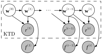
which is essentially the recursive equation of forward probabilities in HMMs. Our model assumes that reward and feedback are conditionally independent given Q-function, i.e.
The graphical model for our algorithm is depicted in Fig. 1.
Our main focus here is on the likelihood of discrete feedback Pr(f (t) ♣s(t) ↪ a(t) ↪w(t) ). In this work, we assume that the feedback is binary (as in [Griffith et al., 2013]), representing whether the last action a(t) executed by the agent was optimal or not, from a potentially imperfect trainer. In a task with M actions, the optimality of an action is equivalent to its Q-value being no less than those of other actions. More formally, action a is optimal if and only if M - 1 dimensional vector d ≥ 0, defined by
where Da is the (M - 1) ⇥M matrix that yields differences in Q-values, e.g. assuming that a = a1,
and q is the M-dimensional vector of Q-values, i.e.
Combining the equations, action a is optimal if and only if
Thus, feedback f from the trainer whether action a is optimal (good) or sub-optimal (bad) is defined using the above:
where ⇢TP and ⇢TN are the true positive and true negative rates of feedback accuracy.
We are now ready to derive posterior over w given feedback, which is shown to be a mixture of two component distributions. As an example, when f = good,
where ⌘ is the normalizing constant and δ is the threshold function. In particular, when the prior on w is the MVN as in KTD, the posterior is the mixture of truncated MVNs. More formally, given prior Pr(w) = N(θ↪ ⌃), the first component distribution becomes
The second component distribution corresponding to the complement of truncation is rather unwieldy, requiring M truncated MVNs to obtain the exact form. However, we can use Eq. (10) and (11) to efficiently compute the moments.
Algorithm 2: KTD update for reward and feedback
Finally, combining the results, the posterior is given by
Thus, we first perform KTD update using reward r(t) , and then use Eq. (12) to update the posterior using feedback f (t) .
The remaining challenge is that the number of mixture components grows exponentially in the number of updates. Although there are a number of techniques to mitigate the problem, our implementation leverages moment matching with a single MVN: we first compute the moments of the two component distributions in Eq. (12) to approximate each of them as MVN, and then compute the moments of the mixture to further approximate it as a single MVN (see Alg. 2).
We note in passing that our probabilistic model of feedback shares similarity with [Boutilier, 2002], where the truncated univariate Normal distribution was used to infer user preferences. In our model, the role of the truncated distribution is different, inferring differences in Q-values for BRL, as well as being extended to multi-dimensional plane truncations.
4 Unknown Feedback Accuracy
In this section, we further extend the algorithm to the case where the agent does not have a-priori knowledge of the accuracy rate of trainer feedback. Given that there is no straightforward conjugate prior for the feedback likelihood and that the accuracy rate is represented by just two parameters ⇢TP and ⇢TN , we can take a simple grid-based filtering approach. Specifically, we prepare N discrete levels of accuracy rates
¶⇢(i) = h⇢(i) T P ↪ ⇢(i) TN i♣i = 1↪ ▷ ▷ ▷ ↪N ⇥N♦ and initialize them with uniform weight !(i) = 1◁N 2 . Upon observing reward and feedback at each time step, we update posterior over w for each ⇢(i) using Alg. 2. Then, weights are updated by
That is, we scale each weight !(i) by factor ⌘(i) = R Pr(w♣r)Pr(f♣w↪ ⇢(i) )dw. The first term Pr(w♣r) of the integrand is the MVN posterior from KTD. The second term Pr(f ♣w↪ ⇢(i) ) is the feedback likelihood, e.g. when f = good for state s and action a,
Thus, we can see that ⌘(i) is the normalizing constant ⌘ in Eq. (12). Combining the results, the weights are updated by
which represents the posterior probability of ⇢(i) .
5 Experiments
Experiments were conducted on the following four RL tasks:
- (a) Inverted pendulum[Lagoudakis and Parr, 2003] is a problem where the objective is to balance a pendulum at the upright position by applying forces to the attached cart. This problem consists of 2 state variables (the angle and the angular velocity of the pendulum) and 3 actions (left force, right force, or no force).
- (b) Mountain car [Sutton and Barto, 1998] is a problem where the objective is to drive an under-powered car up to a hill from a valley as soon as possible. The car must oscillate at the bottom of the valley to gain enough momentum. The problem consists of 2 state variables (the position and velocity of the car) and 3 actions (accelerate forward, accelerate backward, or no acceleration).
- (c) Acrobot [Sutton and Barto, 1998] is a problemwhere the objective is to swing up a two-link under-actuated robot as soon as possible. The first link is suspended from a point and the second can exert torque. Similar to mountain car, it must swing back and forth to gain enough momentum to raise the tip of the second link. The problem consists of 4 state variables (the angle and angular velocity of each joint) and 3 actions (positive torque, negative torque, or no torque).
- (d) Octopus arm [Engel et al., 2005] is a challenging problem where the objective is to control a simulated model of the octopus arm to touch a given target as soon as possible. A detailed description of the model can be found in [Yekutieli et al., 2005]. The problem consists of 82 state variables and 32 action variables. We used the simulation code provided in the 2009 RL competition, which discretized the action space into 8 representative actions 4 .
4 https://code.google.com/archive/p/rl-competition/downloads
| Problem | φ(s↪ a) | dim(w) | Prior w | σr |
|---|---|---|---|---|
| Pendulum | RBF | 25⇥3 | N(0↪ I) | 0.5 |
| Mt. Car | RBF | 25⇥3 | N(0↪ 0▷1I) | 0.5 |
| Acrobot | RBF | 256⇥3 | N(0↪ I) | 0.5 |
| Octopus | RBF | I) | p10 |
Our algorithm, KTD+FB, which extends KTD to learn simultaneously from reward and feedback, is compared to the following algorithms:
- ÷ KTD: A model-free BRL that learns only from reward.
- ÷ Bayesian Q-learning with policy shaping (BQL+PS) [Griffith et al., 2013]: To the best of our knowledge, this is the only BRL algorithm that is capable of learning simultaneously from reward and discrete feedback. However, this algorithm cannot be used directly since it assumes discrete state space to represent policies. Thus, we modified the algorithm to use softmax distribution to represent policies for continuous state space
and to learn policy parameter v by maximizing loglikelihood with an `2 penalty term, given by
where f (⌧) = 1 if the feedback was good and 0 otherwise. We also replaced BQL with KTD since the latter has a more theoretical background. However, note that this extension not only doubles the parameters (w and v), but also requires performing a non-convex optimization at each time step, which incurs a significant amount of computation (LBFGS was used in this paper).
In order to simulate feedback generation, we first obtained reference policy for each problem. For inverted pendulum, we used the straightforward optimal policy as the reference policy: if the pendulum is moving toward the upright position, do nothing; otherwise, apply the force in the reverse direction to prevent the pendulum from falling down. For mountain car and acrobot, we obtained reference policies by running KTD for sufficiently many time steps. For octopus arm, we used a heuristic policy that unfolds arm whenever it is bent and rotates the base towards the target. Then, we generated feedback by comparing the reference policy versus the agent's action and perturbing the feedback signal with parameters ⇢TP and ⇢TN.
Tbl. 1 summarizes the algorithm parameter settings for each problem. Regarding action-selection strategy at each time step, we adopted a simple exploration policy motivated by LinUCB [Li et al., 2010], where we select the action a
| Problem | Known ⇢ (Alg. 2) | Unknown ⇢ (Sec. 4) | KTD (Alg. 1) |
|---|---|---|---|
| Pendulum | 4.09◦0.14 | 4▷73◦0▷13 | 104▷70◦1▷33 |
| Mt. Car | 26.68◦0.33 | 27.03◦0.30 | 6▷62◦0▷19 |
| Acrobot | 13.11◦0.18 | 13.35◦0.12 | 1▷48◦0▷06 |
| Octopus |
5.55◦0.43 2▷38◦0▷36
1▷43◦0▷26
Table 2: Number of finished episodes after initial 2000 time steps (4000 time steps for octopus arm) with feedback from a perfect trainer.
with the maximum index
with c = 2 held fixed throughout time steps. The idea here is that we want to execute the action with the maximally estimated Q-value biased by the confidence in the estimate.
We first compared the learning performance when the trainer feedback was accurate, i.e. ⇢TP = ⇢TN = 1. Fig. 2 shows the results in the first 5000 time steps (12000 time steps for octopus arm). We can clearly observe that providing the agent with accurate feedback enables learning the optimal policy very quickly. In inverted pendulum, the total number of failures of KTD+FB in 5000 time steps was merely 4 on average, and all of them occurred in the very early stage. Although the performance gap between KTD+FB and BQL+PS was very small in acrobot, it was clearly noticeable in other domains. Overall, the performance improvement of KTD+FB over BQL+PS was statistically significant in all problems.
Fig. 3 shows the learning performance of KTD+FB with different feedback accuracy rates in the first 2000 time steps (12000 time steps for octopus arm). We used five accuracy rate settings ⇢TP = ⇢TN 2 ¶0▷5↪ 0▷6↪ 0▷7↪ 0▷8↪ 0▷9↪ 1▷0♦. As naturally expected, the learning performance improved as we increased the feedback accuracy. When ⇢TP = ⇢TN = 0▷5, KTD+FB reduces to KTD with a minor difference due to numerical error. In addition, although not shown in the plots, our algorithm shows symmetric learning performance with an adversarial trainer, i.e. ⇢ < 0▷5. For example, learning performance was same for ⇢ = 0 (a fully adversarial trainer who always lies) and ⇢ = 1.
Tbl. 2 compares the learning performance when the feedback accuracy is known to the agent (Alg. 2) versus unknown to the agent with the accurate trainer. We used the Bayesian filtering algorithm in Sec. 4 with 36 levels of accuracy rates (⇢TP ↪ ⇢TN) 2 ¶0▷5↪ 0▷6↪ ▷ ▷ ▷ ↪ 0▷9↪ 1▷0♦ ⇥ ¶0▷5↪ 0▷6↪ ▷ ▷ ▷ ↪ 0▷9↪ 1▷0♦. The filtering algorithm performed quite well without the information on feedback accuracy, even showing almost same performance in Mountain car and Acrobot.
6 Discussion and FutureWork
In this paper, we presented a model-free BRL algorithm for learning simultaneously from reward and behavior feedback. Our algorithm extends KTD to the setting where the trainer provides, with some error, binary feedback on whether the last action executed by the agent was optimal or not. The probabilistic model behind the algorithm treats the reward from the environment and the feedback from the trainer as two conditionally independent observations generated from the latent Q-value function. At the core of our approach is the generative model of feedback using the MVN with plane truncation, which yields a mixture of truncated MVNs as posterior. We leveraged an efficient technique for computing the first and second moments of truncated MVNs, which allows us to perform m-projection (i.e. moment matching) of the posterior over value functions using a single MVN.


In recent years, there has been a significant growth of interest in (Bayesian) RL agents capable of learning from discrete trainer feedback. One of the ways of achieving this is to use reward shaping [Ng et al., 1999], which requires converting the discrete feedback into numeric values. However, this approach cannot assure that the agent never executes bad actions again as the shaping function only serves as a behavior bias. In addition, this approach generally requires a complete specification of feedback for every state and action before execution, which may be hard to fulfill in practice. Another approach is to use policy shaping [Loftin et al., 2016], which uses explicit models of policies to directly learn from discrete feedback. However, since it is not trivial to reflect reward in learning the policy, an independent model for reward learning is typically used [Griffith et al., 2013]. As a consequence, we cannot readily use Bayes exploration policies [Dearden et al., 1998], such as Value of Perfect Information (VPI), Thompson sampling, or Bayes upper confidence bound in an integrated manner. Our work overcomes these limitations through a probabilistic model that allows us to infer the value function jointly from reward and discrete feedback. Consequently, our agent will never execute bad actions again if the feedback is trusted (unlike reward shaping), and is capable of making better informed choices of actions (unlike policy shaping).
There are a number of directions for future work. First, computing the moments of truncated MVNs requires evaluating the MVN cumulative distribution function. In our case, although we are using thousands of features, the dimension of truncated MVN required to compute moments is effectively reduced to the number of actions. Still, in an environment with a large number of actions, we need a more efficient way of computing moments. In this respect, a low-rank approximation of the covariance matrix may be promising, as well as a variational inference approach. Second, it would be interesting to extend the model to capture the feedback strategy of the trainer as in [Loftin et al., 2016]. Lastly, although we took a grid-based discretization to handle unknown accuracy rate of feedback, a more sophisticated filtering algorithm would be promising.
Acknowledgments
This work was supported by R.O.K. MSIP/IITP (B010116-0307), DAPA/ADD (UD140022PD), U.S. AFOSR, ARO, DARPA, DOT, NSF, and ONR
@inproceedings{ijcai2016p225,
  title     = {Bayesian Reinforcement Learning with Behavioral Feedback},
  author    = {Hong, Teakgyu and Lee, Jongmin and Kim, Kee-Eung and Ortega, Pedro A. and Lee, Daniel D.},
  booktitle = {Proceedings of the Twenty-Fifth International Joint Conference on
               Artificial Intelligence, {IJCAI-16}},
  publisher = {AAAI Press / International Joint Conferences on Artificial Intelligence},
  editor    = {Subbarao Kambhampati},
  pages     = {1571--1576},
  year      = {2016},
  month     = {7},
  url       = {https://ijcai.org/proceedings/2016/225},
}
TY - CPAPER TI - Bayesian Reinforcement Learning with Behavioral Feedback AU - Hong, Teakgyu AU - Lee, Jongmin AU - Kim, Kee-Eung AU - Ortega, Pedro A. AU - Lee, Daniel D. T2 - Proceedings of the Twenty-Fifth International Joint Conference on Artificial Intelligence, IJCAI-16 PB - AAAI Press / International Joint Conferences on Artificial Intelligence PY - 2016 SP - 1571 EP - 1576 UR - https://ijcai.org/proceedings/2016/225 ER -Copied
Machine-readable versions of this paper, for tools and AI agents:





