Class-Wise Supervised Hashing with Label Embedding and Active Bits

1 Introduction

The hashing technique has received more and more attention in large-scale data analytics applications because it can save storage space by mapping each raw data into a binary code and enable fast search. Data-independent hashing methods, such as Locality Sensitive Hashing (LSH) [Gionis et al., 1999; Charikar, 2002], require a long-length binary code to guarantee precision in searching using approximate nearest neighbor (ANN). In order to produce a more compact code, data-dependent hashing methods, known as learning to hash methods [Wang et al., 2016; 2014] have been proposed. Compared to unsupervised hashing methods [Weiss et al., 2008; Liu et al., 2014; 2011; Gong and Lazebnik, 2011], which do not take label information into consideration when learning hash functions, supervised and semi-supervised approaches [Shen et al., 2015; Wang et al., 2010a; 2010b; Liu et al., 2012a; Pan et al., 2015;

Lin et al., 2014] are more promising as they can encode side information for semantic search.

For training hashing functions, most existing supervised and semi-supervised methods [Wang et al., 2010a; 2010b; Liu et al., 2012a; Pan et al., 2015; Lin et al., 2014] rely on an instance-pairwise similarity matrix of labeled training data. The cost in terms of space for generating this matrix is quadratic to the size of the labeled training data. In a large-scale learning problem, the number of labeled training instances can be millions or even billions. In this case, it is impossible to generate a full instance-pairwise similarity matrix for training. As a compromise, sampling techniques are usually adopted to select only a small set of labeled instances to compute the similarity matrix while the remaining labeled instance are discarded [Liu et al., 2012a] or used as "unlabeled data" to construct a regularization term for learning [Wang et al., 2010a; 2010b; Pan et al., 2015; Lin et al., 2014]. However, this may result in information loss for learning semantic hashing functions.

To address the issue mentioned above, in this paper, we propose a class-wise supervised hashing method, which trains a model based on a class-pairwise similarity matrix rather than an instance-pairwise similarity matrix. In many applications, the number of classes is much smaller than that of training instances. Therefore, the storage space for the similarity matrix is dramatically reduced from O(N 2 ) to O(L2 ), where N is total number of labeled instance, and L is total number of classes, which is supposed to be much smaller than N. With the class-pairwise similarity matrix, besides a set of hash functions to map original instances to binary codes 1 , we also aim to learn a class-wise code-prototype for each class with "active" bits.

Our idea is motivated by the example shown in Figure 1, where we are given a set of training instances of four classes: C1, C2, C3 and C4. The goal is to learn three linear hash functions in terms of w1, w2 and w3 to map an instance to a code of three binary bits. Ideally, instances belonging to the same class are expected to have very similar hash codes, while instances belonging to different classes are expected to have very different codes. However, when the number of classes and data size of each class are both large, one may not be able to find a perfect set of hash functions over all the classes through optimization. Suppose the optimal solutions for w1, w2 and w3 are shown in Figure 1(a), where the instances of class C1 are divided by w3 into two areas: A1 and A2, while the instances of class C2 are divided by w2 into another two areas: A5 and A6. Suppose given a query of class C1, which falls in area A2, only instances in area A2 will be turned within Hamming radius 0. If we relax the retrieval condition to be within Hamming radius 1, all instances of C1 (instances in the both areas A1 and A2) will be returned successfully. However, the instances in area A3 of class C3 will be returned as well. Similar situation applies to the retrieval problem of class C2.

1 In this paper, we use +1 and -1 to construct binary codes.

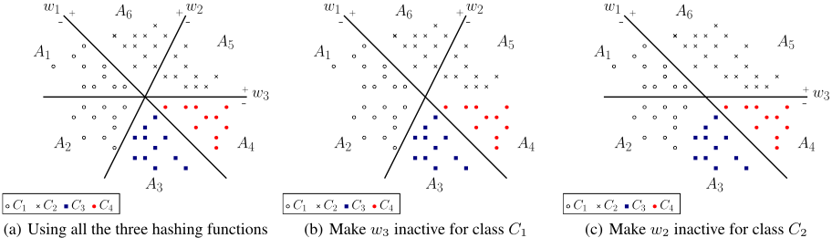
The problem presented above can be solved by introducing a concept of active functions/bits to different class-wise code-prototypes. In the example shown in Figure 1(a), if one defines w1 and w2 to be active functions and w3 be inactive for class C1 as shown in Figure 1(b), then given a query of class C1 that falls in either area A1 or area A2, all instances in class C1 not the other classes will be returned within Hamming radius 0. The case for class C2 is similar if one defines w1 and w3 to be the two active functions for class C2 as shown in Figure 1(c). Note that by introducing active hash functions to different class-wise code-prototypes, the storage of binary codes for training instances can be further saved as for each training instance, one only needs to store those bits that are "active" in the corresponding class-wise code-prototype. For example, for the instances in class C1, only the 1st and 2nd bits are needed to be stored, and the 3rd bit can be discarded.

By summarizing the motivations mentioned above, we come up with a high-level idea on our hashing model design. In order to learn a precise and compact hash code for each instance, we aim to learn a code-prototype for each class, whose length is the same as the number of hash functions to be learned. The constructed code for each instance should be similar to its corresponding class-wise code-prototype. The class-wise code-prototypes should be able to capture the similarity between classes, and are associated with class-specific active bits such that searching is more effective and efficient. In the rest of this paper, we denote by Class-wise Supervised Hashing (CSH) our proposed learning to hash method.

2 RelatedWork

Our work is related to sparse hashing methods [Xia et al., 2015; Masci et al., 2013; Zhu et al., 2013; Wu et al., 2014; Zhang et al., 2016b]. Among these methods, [Zhu et al., 2013; Wu et al., 2014; Zhang et al., 2016b; 2016a] proposed to convert sparse coefficients into 0◁1 binary code or nonnegative integers, which are used to represent the instances based on high-level bases or a dictionary. Such kind of sparse binary codes can be obtained by using 0◁1 instead of -1◁ + 1 for each bit. In other words, the zero-valued bits in [Zhu et al., 2013; Wu et al., 2014; Zhang et al., 2016b] are similar to those of value -1 in our method. We use +1 and -1 to construct binary code and 0 to indicate sparsity of the code. Masci et al. [2013] proposed to add sparsity constraints on the constructed hash codes, while Xia et al. [2015] and Zhang et al. [2016a] proposed to learn a sparse projection matrix for hash functions. These two approaches can both help saving storage space, but to different extents. In general, when the size of training instances is much larger than that of feature dimensions, which is common in many real-world applications, the former approach can save more storage space.

Different from [Masci et al., 2013] to add sparsity constraints on the constructed hash codes for individual instances, our proposed method is able to generate sparse binary codes for labeled training instances through learning a set of class-wise code-prototypes with active bits for different classes. In addition, in most previous methods, the L1 norm is used to induce sparsity, which is a relaxation of the L0 norm, while in our proposed method, we used the L0 norm to control the numbers of active bits for each class-wise code-prototype, and develop an effective algorithm to solve the resultant optimization problem. Note that the concept of active bits was first proposed in [Liu et al., 2012b], where a hash model is learned by exploring the sparse association between hash bits and classes. However, it was specially designed for multilabel classification problems, and fails to be applied to multiclass classification problems as studied in this paper, where the co-occurrence information among classes is not available.

3 Methodology

Assume we are given n training labeled instances ¶(x1↪ y1)↪ (x2↪ y2)↪ ▷▷▷↪ (xn↪ yn)♦, where xi 2 Rd is an input instance, and yi 2 ¶1↪ 2↪ ▷▷▷↪ L♦ is the corresponding class label. Without loss of generality, we assume the input instances to be zero centered, i.e., Pni=1 xi = 0. A hash model aims to map each input instance xi to a binary code of r bits through learning r hash functions as follows,

where each hash function hj(x) is associated with a weight vector wj 2 Rr , andW=[w1↪w2↪ ▷▷▷↪wr]2Rd⇥r is the hash projection matrix. The sgn(x) function is an element-wise sign function defined as sgn(x) = 1 if x ≥ 0, and -1 otherwise. bi2¶1↪-1♦r is the resultant r-bit hash code for xi.

3.1 An Overview of the ProposedMethod

As discussed in Section 1, previous supervised or semisupervised hashing methods aim to enforce the binary codes to be similar (or different) if the corresponding instances belong to the same class (or different classes). One typical approach is to maximize Pni=1 Pnj=1 Kijb>i bj or minimize Pni=1 Pnj=1 ⇣Kij - 1r b>i bj ⌘2 , where K2Rn⇥n is the similarity matrix between instances. When n is large, the cost in terms of both storage and computation is expensive. Though sampling techniques can be applied to approximate the simi-

larity matrix, some label information may be discarded.

To fully exploit all labeled instances to learn hash functions and scale up the learning process at the same time, we propose to learn an additional set of class-wise code-prototypes, denoted by aj (j = 1↪ 2↪ ▷▷▷↪ L), based on a class-pairwise similarity matrix S 2 RL⇥L, where aj is a corresponding r-bit binary code for class j 2 ¶1↪ 2↪ ▷▷▷↪ L♦, and Sjk is positive if classes j and k are similar, otherwise Sjk is negative. Regarding the similarity measure between classes, we can simply define the similarity between class j and itself to be 1, and the similarity between different classes to be -1, i.e., Sjk = 1 if j = k, otherwise, Sjk = -1. When the classes lie in a taxonomy, we can encode the taxonomy structure to construct the class-pairwise similarity matrix. Specifically, motivated by [Weinberger and Chapelle, 2008], we first denote by C a cost matrix with Cjk ≥ 0 being the length of the shortest path between class j and class k in the taxonomy, where j↪ k 2 ¶1↪ ▷▷↪ L♦, and the path is defined to be 0 if j = k. We then normalize the cost matrix by ¯C = D-1◁2CD-1◁2 , where Djj = Pk Cjk is a diagonal matrix. Finally, we define the similarity S with Sjk = -¯Cjk if j 6= k, otherwise, Sjk = 1.

We expect the learned class-wise code-prototypes to have the following properties:

1. Based on the similarity matrix between classes, similar classes should have similar code-prototypes, while dissimilar classes should have different code-prototypes. This can be done by maximizing PLj=1 PLk=1 Sjka>j ak
2. Each class-wise code-prototype aj should be able to guide the learning of hash codes for the instances of class j. This can be done by maximizing Pni=1 a>yi bi, where yi 2 ¶1↪ 2↪ ▷▷▷↪ L♦ is the corresponding class label of bi or xi.
3. Each class-wise prototype-code aj should have its specific active bits. To indicate active or inactive bits, we require aj to be in ¶-1↪+1↪ 0♦r . The l-th bit in aj is active

if its value is nonsparse, i.e., aj[l] = -1 or aj[l] = +1, otherwise, inactive.

3.2 Objective Function

By formulating our high-level ideas described above, we come up with the following objective function,

where bi is a binary code for xi, i = 1↪ ▷▷▷↪ n, while aj is a sparse class-wise code-prototype for class j 2 ¶1↪ ▷▷▷↪ L♦, ayi is the corresponding class-wise code-prototype of xi, S is the class-pairwise similarity matrix, W is the hash projection matrix, ↵ and β are positive tradeoff parameters, k · k0 is the zero-norm that returns the number of nonsparse elements, and m is the parameter controlling the sparsity of each aj .

In the objective of (2), the first term is to enforce ayi and bi to be close to each other. The second term is to ensure that if classes j and k are similar (or dissimilar), the corresponding class-wise code-prototypes aj and ak are similar (or dissimilar). The third term is the negative of a loss function on binary fitting errors, which is commonly used in many learning to hash methods [Gong and Lazebnik, 2011; Shen et al., 2015; Pan et al., 2015; Xia et al., 2015]. The constraint kajk0  m is to enforce each aj to be of at most m active bits.

4 Optimization

To find a feasible solution for the optimization problem (2), in this section, we present an alternating optimization approach.

4.1 W-Step: fix bi and aj, updateW

By fixing bi and aj , the optimization problem (2) becomes

By defining X = [x1↪ x2↪ ▷▷▷↪ xn] and B = [b1↪ b2↪ ▷▷▷↪ bn], the optimization problem (3) can be further rewritten as a regression problem

for which we have the solution,

4.2 B-Step: fixWand aj, update bi

By fixing W and aj , which means ayi is fixed for each xi, and defining a matrix ˆA 2 ¶1↪ 0↪ -1♦r⇥n with the i-th column corresponding to the class prototype ayi of xi, the optimization problem (2) can be reformulated as

where Q(B) = tr( ˆA>B) - β2 ∥∥∥B-W>X∥∥∥2 F . To solve this optimization problem, we further rewrite Q(B) as follows, Since kBk2F and kW>Xk2F are both constant,

where V = ˆA + βW>X. Maximizing Q(B) is equivalent to maximizing tr(V>B). As B 2 ¶1↪-1♦r⇥n , the optimal solution for (5) can be obtained by setting

4.3 A-Step: fixWand bi, update aj

Finally, by fixing W and bi, the optimization problem (2) can be rewritten as follows,

Note that the expression ayi is not consistent with aj. Thus, we need to transform it to aj for convenience in solution induction. To do this, we define ebj as the sum of bi's which belong the j-th class, i.e., ebj = Pi2C bi, where C = ¶i♣yi = j & i = 1↪ 2↪ ▷▷▷↪ n♦. Then (8) can be rewritten as

However, the optimization problem (9) is still difficult to optimize because both the zero-norm constraint (or sparsity constraint) and the discrete constraint on aj are not differentiable. Furthermore, the second term of the objective in (8) is a quadratic term with respect to aj, making it difficult to obtain solutions for all aj at the same time by using the optimization method used in (5).

Alternatively, we propose an algorithm to update only one aj at each time. To avoid confusion, we denoted by at the one to be optimized at each time, and aj, where j 6= t, any one of the remaining constant vectors. Let es be a column vector corresponding to the t-th row of S except for Stt, i.e., es = [St1↪ St2↪ ▷▷▷↪ St↪t-1↪ St↪t+1↪ ▷▷▷↪ StL]>, eA = [a1↪ a2↪ ▷▷▷↪ at-1↪ at+1↪ ▷▷▷↪ aL], and K = ¶1↪ 2↪ ▷▷▷↪ L♦ ∩ ¶t♦. When all ¶aj♦'s except for at are fixed, we can derive that

and

= 2es>eA>at +Stta>t at + const▷ By substituting (10) and (11) into (9), we obtain the optimization problemwith respect to at as follows,

Proposition 1. To solve the maximization problem (12), the number of non-zero elements of at should be maximal. In other words, katk0 = m.

Proof. Define a feasible solution for (12) as ap, where kapk0 = v  m - 1, and another feasible solution as aq, where kaqk0 = v + 1. Assume that these two solutions or vectors are different only on the l-th element, where ap[l] = 0 and aq[l] 6= 0. Let Z(a) = eb>t a + 2↵es>eA>a +↵Stta>a, and

If aq[l] = sgn(u[l]), then Z(aq) - Z(ap) > 1. This means that for any feasible solution ap whose zero norm is less than m, we can always find another feasible solution aq such that Z(aq) > Z(ap). Therefore, the optimal solution for (12) is not ap but the one whose zero norm equals to m.

With Proposition 1, the third term of the objective in (12) equals to a constant ↵ ⇥m. Thus, the objective becomes to maximize eb>t at +2↵es> eA>at or u>at by using the definition of u. It can be shown that the optimal solution is

where ♣u[l]♣ denotes the absolute value of u[l], and ⌘ is the m-th largest absolute value of the elements of u. We can use (13) to obtain solutions for all ¶aj♦'s.

Note that for initialization, we set each class-wise codeprototype aj to be a vector of all zeros. To accelerate the convergence, we initialize the projection matrix W using random sampling from a uniform distribution E(0) as used in LSH.

4.4 Search in Sparse Binary Codes

As discussed in previous sections, the binary codes for instances, ¶bi♦'s, are not constrained to be sparse in training, while the class-wise code-prototypes, ¶aj♦'s, are learned with sparsity constraints. After ¶aj♦'s are learned, for any binary code bi of xi in the database, if its label is known, we can convert it into a sparse version by setting its inactive bits to 0 based on its corresponding class-wise code-prototype ayi .

Note that for search on a database of n non-sparse binary codes of r bits within Hamming radius R, it needs to go through all the hash buckets within R bits of the query binary code [Norouzi et al., 2012]. The number of buckets to be examined is PRi=0 (ri ), and therefore this costs O(r!R!) . In our proposed method, as for each instance, only m active bits needs to be considered, the time complexity for R Hamming radius neighbors search is O(m!R!). If R is not zero, the active bits strategy used in the proposed method will save much retrieval time.

5 Experiment

The datasets we employ to test the performance of the proposed CSH method include the Animals with Attributes dataset 2 (AwA) and the CIFAR-100 dataset [Krizhevsky,

2 http://attributes.kyb.tuebingen.mpg.de/

2009]. AwA consists of 30,475 images of 50 classes of animals, which provides six kinds of pre-extracted feature representations. In our experiments, we use the 4096-dimensional DECAF features, which are obtained via a 7-layer CaffeNet. There is no taxonomy information among classes. However, as all classes are mammal animals, we use part of the Mammals subtrees of WordNet as the taxonomy to construct the class-pairwise similarity matrix. On this dataset, 5% of data (i.e. 1↪ 457 instances) are randomly picked up as queries, and the remained instances form a training set. CIFAR-100 consists of 100 classes with each class containing 600 color images of size 32 ⇥ 32, which results in 60K images in total. In experiments, every image is represented by 512-dimensional GIST features. And 58K instances are randomly selected from the whole set to comprise a training set while the remained 2K instances are used as queries. As only 2-layer taxonomy is provided, in our experiment, we do not encode the taxonomy information into the the similarity matrix for this dataset.

5.1 Methods for Comparison

We compare our proposed CSH method with four hashing methods. They are Locality-Sensitive Hashing (LSH) [Charikar, 2002], Iterative Quantization (ITQ) [Gong and Lazebnik, 2011], Supervised Discrete Hashing (SDH) [Shen et al., 2015] and Supervised Hashing with Kernel (KSH) [Liu et al., 2012a]. The model of LSH is obtained through random sampling. Its performance is guaranteed by probability theory. ITQ is an unsupervised learning method, whose promising performance has been shown compared with other unsupervised hashing algorithms. Therefore, we consider it as a representative for unsupervised hashing. SDH is a recently proposed supervised hashing with a discrete constraint. The discrete constraint is also used in CSH. Though SDH is designed for binary classification, it has shown its effectiveness in ANN search. Moreover, the optimization approach used in SDH is similar to ours. Hence, we choose it as a comparison method. KSH is a famous supervised hashing method based on an instance-pairwise similarity matrix. As the out-of-space issue caused by KSH is the one we aim address in this paper. Therefore, we choose KSH for conducting comparison experiments as well.

5.2 Experimental Setup

In the optimization problem (2) for CSH, there are three parameter ↵, β and m. The tradeoff parameters ↵ and β are to balance the impact of three terms in the objective. The first term is to sum up n items, the second term is to sum up L⇥L items, and the third term is to sum up n items. Suppose each item be equally important in the objective. We set ↵= n◁L2 and β = n◁n = 1. Regarding the sparsity parameter m, we set m= 34 r, where r is the code length. Sensitivity study on different degree of sparsity is also conducted through experiments. For initialization on W in CSH, we adopt the same strategy as LSH. To avoid bias in initialization, we run CSH and LSH 10 times with different random initializations onW3 , and report the averaged results.

Regarding other comparison methods, as "anchors" are required for both SDH and KSH. To avoid bias in anchors selection, we randomly sample 10 different anchor sets from the training data, each of which consists of 1↪ 000 anchors. We run SDH and KSH with the 10 anchor sets, and report the averaged results. In addition, though it has been shown that with only 5% of training data, KSH can still perform well [Liu et al., 2012a], in our experiments, we feed KSH as many training instances as possible for generating the similarity matrix to maximize its performance in terms of search quality. With the computational resources we have, we can generate an instance-pairwise similarity matrix of around 30K instances. Therefore, for KSH, we use all training instances of AwA and 30K training instances of CIFAR-100. Other parameters for the comparison methods are set based on the suggested values reported in the original papers.

5.3 Evaluation Criteria

The mean Average Precision (mAP) is the most popular evaluation criterion for hashing methods [Wang et al., 2010b; Liu et al., 2012a; 2014; Wang et al., 2010a; Gong and Lazebnik, 2011; Shen et al., 2015; Xia et al., 2015; Wu et al., 2013]. Therefore, we adopt it as one of evaluation criteria. However, we find that with binary representations, a lot of instances may have the same Hamming distance to a given query, and thus have the same ranking positions. In this case, mAP scores may be misleading. Therefore, we also use the precision and recall curve within different Hamming radii to a given query to evaluate the hashing performance.

5.4 Comparison Results

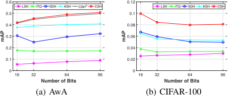
We first compare CSH with the other four hashing methods in terms of mAP in Figure 2. Clearly, CSH outperforms the other baselines with different code lengths on AwA as shown in Figure 2(a). We observe that the three supervised hashing methods, CSH, SDH, and KSH, perform better than the unsupervised methods, ITQ and LSH. This indicate the importance of supervised information for semantic search. Note that CSH without encoding class taxonomy information is also tested on AwA by setting all diagonal entries of the similarity matrix S to be +1, and all the other entries to be -1, which is denoted by CSH0 in the figure. The result reveals that CSH can outperform all other competitors, no matter supervised or unsupervised ones, even without engaging the class taxonomy into learning. The performance of CSH is slightly better than CSH0 , which implies that encoding class taxonomy can help to generate a more precise class-pairwise similarity matrix, and thus improve search quality.

3 In each run, CSH and LSH share the same initialized W.

We also find that the results on CIFAR-100 in terms of mAP are misleading. To be specific, in Figure 2(b), the mAP scores achieved by all the hashing methods are much lower than those shown in Figure 2(a). This implies that learning hash functions on CIFAR-100 is much difficult than that on AwA. In this case, the code of small length, e.g., code of 16 bits, is supposed to perform poor. However, from the figure, the hashing functions with the smallest code length perform best. This is because for a difficult task, with small length of code, a lot of binary codes have the same Hamming distance to a given query. In this case, mAP scores are not reliable.

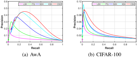
Therefore, we generate the precision-recall curve in Figure 3, where the code length is of 64 bits, and the precision and recall within Hamming radius 2 (PH2 and RH2) are highlighted using circles. In general, the performance is considered to be better if the area under the precision-recall curve is larger. Apparently, CSH performs best on both AwA and CIFAR-100 in terms of the area under the precision-recall curve. Note that the precision-recall curve shown in Figure 3 is quite different from that for information retrieval or classification problems, where the precision would be very high when the recall is close to zero. Here, the precision is low when the recall is close to zero. This phenomenon is reasonable in hashing methods because the Hamming distance between the query and a retrieved instance is discrete, resulting in lots of retrieved instances having the same ranking position. If no retrieved instances have the same code as the query, both the precision and recall are zero, which is the case for LSH and ITQ in our experiments. When retrieved instances have the same code as the query, as some of them may belong to a different class from the query, the precision may not be high, which is the case for KSH, SDH and CSH.

More specifically, as can be seen from results on AwA shown in Figure 3(a), the precision-recall curve of CSH covers largest area. The ranking of the five comparison methods in terms of the area under precision-recall curve is the same as that in terms of mAP. Furthermore, PH2 and RH2 of CSH are much better than the other four methods. From the results on CIFAR-100 shown in Figure 3(b), the precision-recall curve of CSH also covers largest area. Though the precision of KSH is better than CSH when the recall is very low, the gap is not large. Moreover, PH2 and RH2 of CSH are much better than those of the other methods. Except for CSH, RH2s of the other four methods are very close to zero, which means that the codes generated by the these methods on CIFAR-100 are not as compact as CSH. This therefore proves the effectiveness of sparse binary codes constructed by CSH.

5.5 Convergence and Effect of Sparsity Parameter

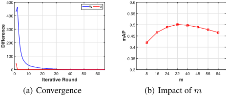
We also conduct experiments on convergence analysis and impact study on the sparsity degree of each ai for CSH. The experiments are done on AwA with the code length fixed to be 64 bits. The convergence analysis on the projection matrix W and the class-wise code-prototypes matrix A is shown in Figure 4(a), where the y axis is the difference in Frobenius norm between two successive iterations. As can be seen from the figure, A converges within 5 iterations, and W begins to converge after 10 iterations, and stays unchanged after 40 iterations. The impact of the sparsity degree on each ai, i.e., the value of m in (2), to the final hashing performance is shown in Figure 4(b), where m varies from 8 to 64 with 8 increment each step. From the figure, we observe that when m is very small, such as m = 8 and m = 16, the mAP score is comparatively low because the number of the active bits may not be sufficient enough to capture important information. When m becomes larger, such as m = 56 or m = 64, the mAP scores drop as most binary codes become "active". This reveals the importance of inactivating a certain number of bits to improve the performance, which is illustrated by Figure 1. These experimental results suggest us to choose the value of m in the range of [ 38 r↪ 34 r], where r is the length of a code.

6 Conclusion

In this paper we propose a novel class-wise supervised hashing method, denoted by CSH. Instead of using an instancepairwise similarity matrix, CSH is based on a class-pairwise similarity matrix. With the class-pairwise similarity matrix, a set of class-wise code-prototypes with class-specific active binary bits are introduced to help generating more compact hashing functions, and thus enable more effective and efficient search. Experimental results verify the superiority of CSH in terms of search quality and storage space over other baseline hashing methods.

Acknowledgments

This work is supported by the NTU Singapore Nanyang Assistant Professorship (NAP) grant M4081532.020.