Change Detection Using Directional Statistics

1 Introduction

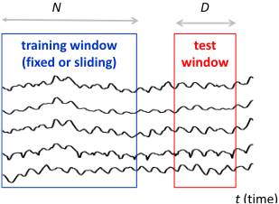
The problem we wish to solve is change detection of multivariate time-series data. Figure 1 shows a typical setting, where our task is to compute the degree of change, or the change score, of the data within the test window taken at time t in comparison to the training window.

The task of change detection has a long history in statistics. The standard strategy is to use a parametric model for probability density and compute the likelihood ratio to quantify the degree of change between fitted distributions [Chen and Gupta, 2012]. For a concise review from a statistical machine learning perspective, see [Yamada et al., 2013].

When applying a change detection method to real-world problems, the major requirements are interpretability and robustness to nuisance noise variables. To validate detected changes with domain knowledge, it is almost always required to explicitly present statistics (or feature) for the parametric model, such as the mean for Gaussian. Although it is possible to design an algorithm that skips the explicit step of feature extraction and jumps directly into score calculation [Liu et al., 2013], such an approach is not highly appreciated in practice due to the lack of interpretability. In the multivariate setting, the robustness to noise variables is the other critical requirements since changes may not always occur in all of the variables simultaneously. In fact, under the existence of nuisance noise variables, the performance of direct density-ratio estimation approaches is known to significantly degrade [Yamada et al., 2013].

Considering these two requirements, we focus on change detection approaches having explicit two steps of feature extraction and score calculation. There are two important decision points here: (1) Parametric model for probability density function, and (2) scoring model for the change score.

In this paper, we propose a novel framework for change detection for multivariate sensor data. Our contribution is threefold:

• ÷ We develop a novel feature extraction method based on regularized maximum likelihood of the von MisesFisher (vMF) distribution.
• ÷ We show that the feature extraction method is reduced to an optimization problem called the trust-region subproblem [Tao and An, 1998; Hager, 2001].
• ÷ We propose a novel scoring method based on a parametrized Kullback-Leibler (KL) divergence.

Implications of these contributions are as follows. First, our feature extraction method is the first proposal to efficiently remove the multiplicative noise that is ubiquitous in many physical systems. Thanks to an `1 regularization scheme, it is also capable of automatically removing samples contaminated by the unwanted noise. Second, the trust-region subproblem guarantees the global optimality in a certain limit, which is especially important for noisy data. Third, the parametrized Kullback-Leibler divergence for scoring provides us with a trustworthy way to quantify the discrepancy between different subspaces with different dimensionalities.

2 Extracting feature matrix from noisy data

The proposed method consists of two steps. The first step computes an orthonormal matrix as the signature of the fluctuation patterns of multivariate data. The second step computes the difference between two data sets in the past and present through the computed orthonormal matrices. This section explains the first step.

2.1 The vonMises-Fisher distribution

Assume we are monitoring a system with M sensors, and we are given N measurements ¶x(1) ↪ ▷ ▷ ▷ ↪ x(N) 2 RM ♦, which may correspond to either the training or the test window in Fig. 1. Our principal probabilistic model is the von MisesFisher (vMF) distribution [Mardia et al., 1980]:

where IM◁2-1(·) denotes the modified Bessel function of the first kind with the order M2 - 1. The random variable z is assumed to be normalized in the sense z>z = 1, where > represents transpose. The vMF distribution has two parameters: the mean direction u and the concentration parameter . As these names suggest, the vMF distribution describes random variability of the direction around the mean vector.

The intuition behind the use of vMF distribution is as follows. When describing the measurements using the vMF distribution, we look only at the direction, disregarding fluctuations along the direction. This automatically gives the robustness to multiplicative noise, which is quite common in practice in systems with redundancy. As an example, we will look at an ore transfer system, where two belt conveyors are operated by the same electronic system. In this system, major fluctuations in one system due to e.g. dynamic load changes are shared by the other system. In systems having strongly correlated variables, the vMF distribution can be a more natural tool for systemmonitoring than the Gaussian.

2.2 Weighted joint maximum likelihood

To simplify the notation, we introduce the data matrix

where kz(n) k2 = 1 and b(n) ⌘ kx(n) k2 for n = 1↪ ▷ ▷ ▷ ↪N and k·kp being the p-norm. The parameters of the vMF distribution may be inferred by maximizing a likelihood function:

where we introduce sample weights w ⌘ (w(1) ↪ ▷ ▷ ▷ ↪ w(N) )>. We wish to capture major patterns represented as the directional data by optimally choosing the weights so that less trustworthy samples are down-weighted.

The weighted likelihood L(u↪w♣X) has only a single pattern u, and naively maximizing L(u↪ w♣X) produces only the single direction. To capture multiple patterns of the change, we jointly fit m different distributions while keeping the overlap minimal by imposing the orthogonality between different patterns:

where Im is the m-dimensional identity matrix, U ⌘ [u1↪ ▷ ▷ ▷ ↪um], and W ⌘ [w1↪ ▷ ▷ ▷ ↪wm]. The term R(W) is a regularizer to remove the trivial solution on the sample weights. Here we consider the elastic net regularization [Zou and Hastie, 2005]:

where λ and ⌫ are given constants, typically determined by cross-validation.

The first term of the objective function is given by

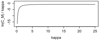
where we defined γ ⌘ ln cM(), b ⌘ [b(1) ↪ ▷ ▷ ▷ ↪ b(N) ]>, and 1 is a column vector of all ones. Throughout the paper we will treat  as a given constant. Fortunately, γ◁ is quite insensitive to , as shown in Fig. 2. One useful heuristic is simply to set  = M. Otherwise, we can use known approximation algorithms given in [Sra, 2012].

2.3 Iterative sequential algorithm

The optimization problem (5) can be sequentially solved for each of (ui↪wi). Imagine that the sample weight w is initialized to a vector. Given w, Eq. (5) is reduced to

for the first u. The solution is readily obtained as

Given this solution, the problem (5) for w is now written as where q is defined byq ⌘ γb + X>u▷

This problem is a special case of LASSO regression, and has a closed-form solution [Wen et al., 2010] as

where ⊙ denotes the componentwise product, 0 is the zero vector, and ♣q♣ is an N-dimensional vector whose n-th entry is ♣qn♣. With this new w, we can solve Eq. (8) again. We repeat solving Eqs. (8) and (10) alternatingly until convergence.

Once we get the first solution (u1↪ w1), we move on to the next solution. We again start with initialized w and solve the following problem instead of Eq. (8):

By introducing Lagrange multipliers ↵↪ β1 for the two constraints, respectively, we have the condition of optimality as

Using the constraints, the candidates for the solution are

There are two stationary points, and by plugging them into the objective function in Eq. (13), we can get the optimal solution u⇤ . This solution is inserted into Eq. (10) to get a new w. These steps are repeated until convergence.

It is straightforward to generalize the above procedure for j = 2↪ ▷ ▷ ▷ ↪m. We summarize the procedure in Algorithm 1, which we call the REgularized Directional feature extraction (RED) algorithm:

Algorithm 1 RED algorithm.

Input: Initialized w. Regularization parameters λ↪ ⌫. Concentration parameter . The number of major directional patterns m.

while no convergence do

end while

end for Return U and W.

In Eq. (17), we define Uj-1 ⌘ [u1↪ ▷ ▷ ▷ ↪uj-1]. IM is the M-dimensional identity matrix. The complexity of RED algorithm for each while loop iteration is O(NM).

3 Theoretical analysis

3.1 Convergence of RED algorithm

We have the following convergence theorem:

Theorem 1. Define g(w↪ u) ⌘ u>Xw + γw>b - R(w). The sequence ¶g(wj↪uj)♦j=0↪1↪▷▷▷ generated by the whileloop of Algorithm 1 has a finite limit.

Proof. First, we prove that the sequence ¶g(wj↪uj)♦ is bounded above. We have

We have

where σmax is the nonnegative maximum eigenvalue of XX>. The inequality (21) is due to λ and ⌫ being positive, the last inequality (22) is derived from kuk2 = 1.

where the first inequality comes from Step 1, the last one is due to Step 3. The boundedness and monotonically increasing of the sequence ¶g(wj ↪ uj)♦ complete the proof.

3.2 Global optimality in ⌫ ! 0

Here we look at the following theorem:

Theorem 2. When ⌫ tends to 0, the nonconvex problem (5) is reduced to an optimization problem in the form of

which has a global solution obtained in polynomial time.

Proof. The non-convex optimization problem (23) is known as the trust region subproblem. For polynomial algorithms to the global solution, see [Sorensen, 1997; Tao and An, 1998; Hager, 2001; Toint et al., 2009]. Here we show how the algorithm is reduced to the trust region subproblem.

When ⌫ = 0, the objective function (5) leads to the optimality condition w.r.t. w as

which immediately gives an analytic solution as w = q◁λ. By inserting this solution into the objective function in Eq. (5), we have an optimization problem only for u:

Let u1 be the solution of this problem. Once u1 is obtained, we again solve another trust-region subproblem of the

which is obviously equivalent to Eq. (23) with Q ⌘ XX> 2 RM⇥M and c ⌘ 2γXb 2 RM .

form (23) but in the RM-1 space by adding an orthogonality condition u>1 u = 0. In particular, without loss of generality, we assume the last component of u1 is nonzero, i.e., u1↪M 6= 0. Define y = (u1↪ ▷ ▷ ▷ ↪ uM-1) and a = (u1↪1↪ ▷ ▷ ▷ ↪ u1↪M-1). The problem (23) with the additional linear equality constraint is equivalent to

Consider the Cholesky decomposition for rank-one update

and the change of variable y = L>(u1↪ ▷ ▷ ▷ ↪ uM-1)>. The decomposition can be done efficiently, for example [Gill et al., 1974]. The problem (24) is rewritten as

which has exactly the same format with (23).

When more than two orthonormal vectors ui are needed, a set of linear equations is additionally considered

A variable elimination method can be used in order to work on a reduced space. Note that an eigenvalue decomposition for a matrix of dimension M-j is needed to transform it into a (M - j)-dimensional trust region subproblem. In this way, we have a set of orthonormal vectors ¶u1↪ ▷ ▷ ▷ ↪um♦, where m is an input parameter representing the number of major directional patterns.

Although the global optimality is no longer guaranteed when ⌫ > 0, we can take advantage of the global solution at ⌫ = 0 to initialize w in Algorithm 1. In practice, if there is a concern about the quality of the solution, we can gradually increase the value of ⌫, and use the obtained ¶wj♦'s for the next trial for a larger ⌫. Although mathematically the RED algorithm is an iterative algorithm that may be trapped by sub-optimality, we can loosely say that it is an "almost guaranteed" algorithm in practice.

4 Parameterized KL divergence for scoring

Solving the optimization problem for the training and the test windows, we obtain two sets of orthonormal vectors ¶u1↪ ▷ ▷ ▷ ↪ um♦ and ¶v1↪ ▷ ▷ ▷ ↪ vr♦ where m and r are the number of vectors given as input parameters. Computing the change score amounts to evaluating the dissimilarity between the two vector spaces specified by orthonormal matrices

Now our problem is to compute the dissimilarity on a Stiefel manifold, which is the space spanned by orthogonal matrices.

As illustrated in Fig. 1, in practice, the window size D should be chosen as small as possible to minimize the time lag in change detection, while the number of samples N in the training data should be large enough to make sure to capture major patterns. Depending on the nature of data, it makes sense to assume m 6= r.

To handle this general situation, we consider linear combinations of ui's and vi's and define the change score as a parameterized version of KL divergence:

under the constraint of f >f = 1↪ g>g = 1. This can be also viewed as an averaged version of the log likelihood ratio, which is the standard measure of change detection [Chen and Gupta, 2012].

By inserting the definition of the vMF distribution in Eq. (1), we have

where h·i is the expectation w.r.t. M(x♣Uf↪ ). Since hxi / Uf follows from the basic property of the vMF distribution [Mardia et al., 1980], we have

where we dropped an unimportant prefactor.

Solving the optimization problem (28) is easy. Introducing Lagrange multipliers ⇡1↪ ⇡2 for the two constraints, it is straightforward to obtain optimality conditions as

This means that f and g are found via singular-value decomposition of U>U(t) , which is a small matrix of size m⇥ r. The maximum of the objective function is simply given by the maximum singular value, σ(t) 1 ; thereby we reach the final formula for the change score:

The maximum singular vector is efficiently computed by the power method [Golub and Loan, 1996]. In most practical situations, it requires only iterations as many as min¶m↪ r♦. The complexity to compute the KL-based change score is (min¶m↪ r♦)3 . Since m and r can be just several in most applications, it is negligible in practice.

5 Related work

As described so far, the proposed method extensively uses the vMF distribution. For change or anomaly detection, little work has focused on the vMF distribution . [Id´e and Kashima, 2004] seems to be one of the earliest pieces of work that explicitly leverages the vMF distribution for anomaly detection, but it does not discuss the particular task of change detection and sample regularization.

In statistics, a lot of efforts have focused on asymptotic analysis of the likelihood ratio [Chen and Gupta, 2012]. Recently, [Kuncheva, 2013] compares various change detection approaches and concludes that a model combining Gaussian mixture and Hotelling's T 2 statistic works best. However, it is widely known that stably learning Gaussian mixture is hard for physical sensor data we are interested in, which is quite noisy and includes many outliers. Also, in general, accurately estimating densities itself is challenging when dimensionality is high (M & 10).

To address the challenge of density estimation, [Kawahara and Sugiyama, 2009; Liu et al., 2013] proposed an interesting technique of direct density-ratio estimation, which integrates the two steps of parametric model estimation and scoring into a single step of density-ratio estimation. Thanks to the integration of the two steps, their approach is generally better than those estimates two densities individually. However, due to the very same reason, they lack practical interpretability, which is of critical importance in practice. Also, it has been pointed out that the performance significantly degrades when some of the variables are just non-informative nuisance features [Yamada et al., 2013].

Recently, to extract the most informative features from multivariate time-series data, [Blythe et al., 2012] proposed an interesting approach called stationary subspace analysis (SSA). Although SSA proposed for the task of time-series segmentation, which is different from the on-line changedetection we are dealing with, we experimentally compare it with the proposed method in the next section.

6 Experimental results

6.1 Methods compared

We compare the proposed method denoted by RED+KL, which uses Algorithm 1 for computing U and U(t) in Eqs. (25) and (29) for the change score, with the following alternative methods:

• ÷ RED+tr: Use Algorithm 1 for U but replace Eq. (29) with the trace norm where r = m:

• ÷ SSA: Use SSA for U. First identify the most stationary subspace by solving

where E is the number of epochs defined by a nonoverlapping time window of size D, and ¶θi↪⌃i♦ are the sample mean and covariance matrix computed in the i-th epoch. ♣ · ♣ represents the determinant in this case. Once V is found, U is obtained as the complement space of V. The change score is computed by

where θ(t) and ⌃(t) are the mean and the covariance matrix over D(t) , which is defined as the set of the samples in the sliding window at time t. Before computing these, the data is whitened with the same pooled mean and covariance of the training data.

• ÷ PCA: Use the principal component analysis for U. Employ the mean reconstruction error for scoring [Papadimitriou and Yu, 2006] :

• ÷ T2: Use the mean Hotelling's T 2 statistic

for scoring. Here θ and ⌃ are the mean and the covariance matrix of the training data. T2 is compared only in change detection since it has no explicit feature extraction step.

6.2 Synthetic data: comparison of feature extraction methods

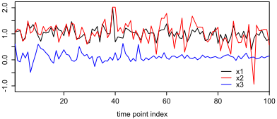
Figure 3 shows three-dimensional synthetic time-series data we generated. In this data, x1 and x2 are quite noisy but significantly correlated, while x3 is uncorrelated to the others. Thus we expect the principal direction would point to the 45◦ line between x1 and x2.

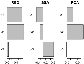
We compared the proposed algorithm (denoted simply by RED) with two alternatives SSA and PCA. All methods take the data matrix X as the input, and return an orthonormal matrix U as the output. Figure 4 shows the coefficients of the first component u1. For RED, we used (λ↪ ⌫) = (1↪ 4), while for SSA we used D = 25.

We see that RED successfully captures the expected 45◦ direction as the principal direction. PCA has a similar trend, but due to the major outlier in x2 at 94 (see Fig. 3), it has more weight in x2. Close inspection shows that RED automatically removes this outlier by putting zero weight, demonstrating the automated noise-filtering capability.

The basic assumption of SSA is that the stationary components are most likely noise, and the non-stationary components are more informative for change detection. In this particular example, the major pattern is the correlation structure between x1 and x2, and the other variable x3 is the noise. However, due to the heavy noise especially in the first half of x3, SSA fails to disregard the noise variable.

6.3 Real-world data: comparison of on-line change detection performance

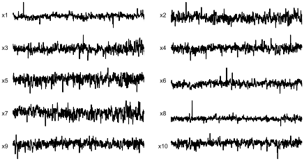
We applied the proposed method to a real-world on-line change detection task. Figure 5 shows time-series data from an ore transfer system being monitored by ten sensors measuring physical quantities such as speed, current, load, temperature, and displacement. The data itself was generated by a testbed system to simulate the normal operating condition and thus used as the training data. As introduced in Sec. 2.1, the system consists of two almost equivalent subsystems, and some of the variables are significantly correlated, and incur the multiplicative noise. As seen, the data is extremely noisy and sometimes exhibits impulse-like noise due to the physical operating condition of the outdoor ore transfer system.

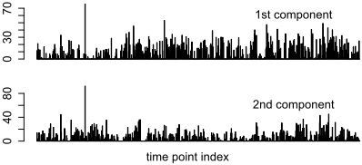
For this training data, we applied the RED algorithm to find U and W. Figure 6 shows W = [w1↪w2], where we used (λ↪ ⌫) = (2↪ 9) that maximized the F score for the test data (see the next paragraph). We see that many samples are driven to zero. In fact, 43 and 39 percents of the samples have exact zero in w1 and w2, respectively, out of which about 16 percent are zero in both. Close inspections show that almost all of "out-of-context" outliers are cut off, while informative outliers that are consistent to the major correlation structure survive. This is exactly what we expected.

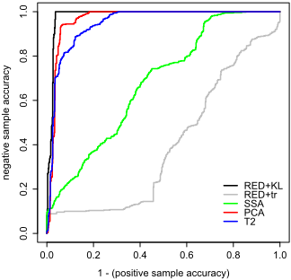
We evaluated the performance of on-line change detection using another data set, where changes due to system malfunctions are recorded. Most of the failure symptoms are associated with unreasonable changes in the correlation structure between the variables. We simply use the negative-sample and positive-sample accuracies as the performance metric. Here, the negative samples are defined by those not belonging to change-points, while the positive samples are those belonging to change-points. We used the harmonic average (F score) of them to determine the (λ↪ ⌫) values. We use the window of D = 60 over about 1200 samples. Figure 7 compares the ROC curve. Clearly, RED-KL with (m↪ r) = (2↪ 3) outperforms the alternatives. It is interesting to see RED-tr gives the worst, which demonstrates the importance the proposed subspace comparison technique of Eq. (29). For this data set, SSA fails to capture change points. The main reason is that SSA is not necessarily robust to spiky outliers as seen in Fig. 5. Since the correlational structure is critical to detect change points in this data, it makes sense that the PCA and T2 do a good job.

7 Conclusion

We have proposed a new on-line change detection algorithm for multivariate time-series data. Our algorithm extracts major directional patterns while automatically disregarding less informative samples. We proved the convergence of the algorithm, and showed that the quality of the solution is supported by the global optimality of the trust-region subproblem. We also proposed a new method of scoring the change based on a parameterized KL divergence. We validated the algorithm using real-world data.