On Structural Properties of MDPs that Bound Loss Due to Shallow Planning

1 Introduction

Planning in Markov Decision Processes (MDPs) involves a lookahead at the consequences of potential action choices using a computational-model of the transition dynamics and the reward function components of the MDP. The horizon specified as part of the planning problem determines how deep (far into the future) the lookahead has to be. The longer the planning-horizon the greater the computational effort needed to compute an optimal policy. To save on this computational effort, planners often use a smaller than specified planning horizon; hereafter we refer to this as shallow planning. Of course, the computation saved by shallow planning comes at the cost of obtaining a policy that is suboptimal relative to the optimal policy. Recent work by Jiang et al. [2015b] shows that when planning with inaccurate models (perhaps learned from small amounts of data) it can actually be beneficial to use shallow planning because it avoids overfitting to the noise in the inaccurate model. In this paper, we focus exclusively on the setting of planning with accurate models with the goal of understanding what properties of the MDP help determine the loss due to shallow planning.

A widely understood but coarse upper bound (see Equation 2) on the loss due to shallow planning is outlined below; it is based only on the largest reward in the MDP and does not exploit any other finer-grained properties of the MDP. In this paper, we identify a set of structural properties of an MDP some of which depend on the reward function alone, some on the transition dynamics alone, and some that depend on the interaction between rewards and transition dynamics. We provide planning loss bounds in terms of these structural parameters and, in some cases, also show tightness of the upper bounds. Empirical results with randomly generated MDPs are used to validate qualitative properties of our theoretical bounds for shallow planning.

2 Planning Setting &Notation

An MDP is specified as a tuple M = hS↪A↪ P↪R↪ γevali where S is the state space; A is the action space; P : S⇥A⇥S ! [0↪ 1] is the transition function, and R : S⇥A ! [0↪ Rmax] is the reward function. The evaluation discount factor, γeval 2 [0↪ 1), determines the effective planning horizon of the problem (more on this below). The planning task is to compute an optimal policy, a mapping from states to actions, that maximizes value, that is the expected sum of future rewards discounted by γeval at every time step. Given a policy ⇡ : S ! A, we use V ⇡M↪γeval (s) to denote its value as a function of the starting state s (with a slight abuse of notation we will also treat V ⇡M↪γeval as a vector in R♣S♣ ). Given an MDP, there always exists a policy that simultaneously maximizes the value of all states, and we denote such an optimal policy as ⇡⇤M↪γeval .

Throughout this paper we will use the phrases "discount factor" and "planning horizon" interchangeably, since the infinite sum of rewards discounted by γeval are approximated by a finite horizon of order O(1◁(1 - γeval)) in online planning algorithms such as Monte-carlo Tree Search methods [Kearns et al., 2002]. In practice, to save computational costs a shallow planner would use a discount factor γ < γeval to guide the planning algorithm in its computation/search of a good policy. We emphasize that the ultimate goodness of the policy ⇡ found by the shallow planner will still be evaluated in M using γeval. To facilitate analysis, we ignore details of specific shallow planning algorithms and instead assume perfect planning under γ, i.e., we assume the shallow planning algorithm outputs ⇡⇤M↪γ , the policy that is optimal in M for a discount factor γ. We define the loss due to shallow planning as the worst (over all states) absolute difference in value of the optimal policy ⇡⇤M↪γeval and ⇡⇤M↪γ , i.e., Finally, because we only consider planning with accurate models, hereafter we drop explicit dependence on M in all notation (for value functions and policies) unless otherwise specified, for they are all automatically with reference to the true MDP M.

3 Structural Parameters that Bound Loss

Before we turn to our finer-grained parameters that bound loss due to shallow planning, we note here that there is a straightforward bound on loss that comes simply from the largest reward (this has been explicitly given by Petrik & Scherrer [2009]; we derive it in Section 3.2 for completeness):

This bound ignores the role of transitions in determining value functions, and indeed any other aspect of reward functions but its largest value, and finally any interaction between rewards and transitions.

3.1 Value Function Variation Parameter &Loss

We begin with a summary "intermediate" parameter and a bound on the loss derived from it; later we show how to relate this summary parameter to several high-level properties of an MDP that pertain to rewards, transitions, and their interaction.

For (environment M and) discount factor γ the valuefunction-variation parameter, γ , measures the maximal variation in optimal value between any two states, or equivalently how much difference the choice of start state can make on the value an agent can achieve. Note that the quantities in γ depend only on γ and not at all on γeval. Next we use this parameter to bound the loss defined in Equation 1 as follows.

Theorem 1 (Upper-Bound on Loss from γ).

Proof. First notice that

On the right-hand side of the equations, each column of the array forms a geometric series with ratio γ. This means that for any policy ⇡, as we show below, V ⇡ γeval can be written as a linear transformation of V ⇡ γ by re-arranging the reward obtained at each step: 8s 2 S, let es be the unit vector with the element indexed by s equal to 1, we have

where [P ⇡ ] is a ♣S♣ ⇥ ♣S♣ matrix with the element indexed by (s↪ s0 ) being P(s0 ♣s↪ a), and R⇡ is a ♣S♣ ⇥ 1 vector with the s-th element being R(s↪ ⇡(s)). Then, the value difference: 8s 2 S,

The first inequality above holds by optimality of ⇡⇤ γ for discount factor γ and the second inequality holds because for any stochastic vectors p↪ q, we have ♣p>V ⇡⇤ γ γ -q>V ⇡⇤ γ γ ♣  γ.

3.2 Bounding Value Function Variation using other parameters

Here we develop several structural parameters that bound γ.

Rewards-Only Parameters

The first rewards-only parameter is simply the largest reward. Proposition 1 below shows how it can be used to bound γ (the proof is straightforward and hence omitted) and when this is applied to Theorem 1 we get the known bound on loss due to shallow planning in Equation 2.

Proposition 1. γ  Rmax◁(1-γ).

The next rewards-only parameter stems from the observation that if we were able to obtain Rmax immediate reward in every state, there would be no need to plan ahead. In general, we show that the loss of shallow planning can be bounded by the extent to which this criterion is violated.

Definition 2 (Reward Variation).

Proposition 2. γ ∆R◁(1-γ).

Proof. The myopic policy s 7! argmaxa R(s↪ a) yields at least mins maxa R(s↪ a)◁(1 - γ) value from any starting state, which is a lower bound on V ⇡⇤ γ γ . On the other hand, any policy and starting state pair cannot have value more than maxs↪a R(s↪ a)◁(1-γ), and the proposition follows by combining the two bounds.

Worst case tightness We show that the planning loss bound based on ∆R by combining Theorem 1 and Proposition 2 is tight in the worst case (and so is Theorem 1 itself, as a direct corollary).

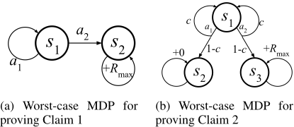
Claim 1. For any ∆R 2 [0↪Rmax], γ 2 [0↪ 1 -∆R◁Rmax], γeval 2 [γ↪ 1), there exists an MDP M with reward variation ∆R, and the loss incurred by using γ is equal to the bound given by Theorem 1 and Proposition 2.

Corollary 1. For any γ 2 [0↪Rmax]↪ γ 2 [0↪ 1)↪ γeval 2 [γ↪ 1), there exists an MDP with value function variation γ and the loss incurred by using γ is equal to the bound given by Theorem 1.

Proof of Claim 1. Consider the 2-state MDP shown in Figure 1a: state s2 is absorbing with reward Rmax; state s1 has two actions, with a1 keeping the agent in state s1 and giving reward R(s1↪ a1) = r, and a2 transitioning to s2 with reward R(s1↪ a2) = (r - γRmax)◁(1 - γ). It is easy to verify that R(s1↪ a2)  R(s1↪ a1), hence ∆R = Rmax - r. The MDP is designed so that ⇡⇤ γeval (s1) = a2 and ⇡⇤ γ (s1) = a1, and so the loss at state s1 of using γ is (Rmax-r)(γeval-γ) (1-γ)(1-γeval) , which is exactly equal to the bound since Rmax-r 1-γ = ∆R◁(1 - γ) = γ .

Transitions-Only Parameters

By using structure in the transition probabilities we can get tighter bounds on γ. The next parameter, ✏-mixing time, is motivated by the fact that if the MDP mixes fast under a policy ⇡, then the value function of ⇡ has small variation over the state space. When ⇡ = ⇡⇤ γ , the parameter yields a bound on γ (explicitly stated in Corollary 2). For ease of technical presentation we will assume that the Markov Chain induced by all policies we consider is ergodic (i.e., under any policy, it is possible to reach any state from any other state).

Definition 3 (✏-mixing time). Define the ✏-mixing time for policy ⇡ as

T⇡(✏) = inf {T : 8s 2 S↪ t ≥ T↪ ∥∥e>s [P ⇡ ]t - (⇢⇡ )>∥∥1  ✏ where ⇢⇡ is the limiting distribution independent of the starting state.

Proposition 3. For policy ⇡,

To prove Proposition 3, we first prove the following lemma, which is widely used in the MDP approximation literature.

Lemma 1. Given stochastic vectors p↪ q 2 R♣S♣ , and a real vector V with the same dimension,

Proof. Let c = (maxs V (s) +mins V (s))◁2, and 1 be the ♣S♣ ⇥ 1 all-1 vector,

Proof of Proposition 3. We reduce Proposition 3 to Proposition 5 (presented below): if ⇡ has ✏-mixing time T⇡(✏) w.r.t. ⇢⇡ , we have for any t ≥ T⇡(✏)↪ s 2 S,

Therefore T⇡(✏) is also an (✏Rmax◁2)-return mixing time for ⇡, and applying Proposition 5 the result follows.

The next transition-only parameter is the stochastic diameter TM, the longest expected time to travel from one state to another. If this parameter is small, V ⇡⇤ γ γ must have a small variation, otherwise we could improve the value of lowvalued states by a non-stationary policy that travels to a highvalued state first and executes the optimal policy afterwards.

Definition 4 (Stochastic diameter).

Proof. It suffices to show that for any s↪ s0 2 S, V ⇡⇤ γ γ (s0 ) - V ⇡⇤ γ γ (s)  1-γ TM 1-γ Rmax. Since ⇡⇤ γ is optimal under γ, we can lower bound V ⇡⇤ γ γ (s) by the value obtained by starting at s and following any policy. In particular, consider a nonstationary policy that first travels to s0 by executing the policy that achieves the minimum in the definition of TM, and then switch to ⇡⇤ γ . Suppose it takes t steps to get to s0 (t is a random variable), then the non-stationary policy gives at least γ tV ⇡⇤ γ γ (s0 ) value, and

Transitions-and-Rewards Parameters

Thus far, we have provided parameters of rewards alone and transitions alone. Here we consider a parameter that captures the interaction between rewards and transitions, the ✏-return mixing time, which measures mixing via the closeness of the expected reward obtained after a particular time step and that obtained in the long run. 1

Definition 5 (✏-return mixing time).

Proposition 5.

Proof of Proposition 5. Let V ⇡γ = V ⇡ γ - γ T v ⇡ (✏) 1-γ ⌘⇡ 1, which is the value function offset by a state-independent constant. For any s↪ s0 2 S, V ⇡ γ (s) - V ⇡ γ (s0 ) = V ⇡γ (s) - V ⇡γ (s0 )↪ and V ⇡γ is equal to

1 This definition is slightly adapted from Kearns & Singh [2002], who considered the average reward obtained in first T time steps.

We now have,

4 Action Variation

In the preceding section, we looked at structural parameters of the MDP that bound the loss due to shallow planning, all via an intermediate quantity γ that characterizes the value function variation. Yet, there are MDPs with large γ that still have a small loss. While covering all such cases is outside the scope of this paper, we cover one such class of MDPs. Namely, those MDPs where different actions at the same state have almost identical distributions over next-states; no deep planning is needed in these MDPs as they are essentially contextual bandits (with Markovian, not i.i.d., contexts). We introduce the notion of Action Variation to capture this idea, and provide an associated loss bound which subsumes Theorem 1.

Definition 6 (Action Variation).

Theorem 2.

Theorem 2 is a planning loss bound that depends on both δP and γ; the bound monotonically increases with δP and reduces to Theorem 1 when δP takes the maximal value 2.

To prove the theorem, we first define the commonality between two probability distributions, and state a key lemma w.r.t. this quantity. Note that commonality appears in the mixing time literature for Markov chains in linking the notions of total variation and coupling [Levin et al., 2009, Section 4.2].

Definition 7. Given two vectors p↪ q of the same dimension, define comm(p↪ q) as the commonality vector of p and q, whose s-th element is comm(s; p↪ q) = min¶p(s)↪ q(s)♦▷

Lemma 2. Suppose p and q are stochastic vectors over S, 8⇡1↪ ⇡2 : S !A,

Proof of Lemma 2. Let P ⇡ (s♣·) be a column vector of transition probabilities from each state to s under policy ⇡, then

Define z as comm(p↪ q) normalized so that kzk1 = 1, then

The last step uses the fact that k · k1 is a convex function, and each row of P ⇡1 - P ⇡2 has `1-norm bounded by δP .

Proof. Using Fact 1, the LHS is

Proof of Theorem 2. The proof follows from the proof for Theorem 1 up to Equation 3. The k-th term in the summation is (ignoring a factor of (γeval - γ)γeval k-1 for the moment):

Summing over k = 1↪ 2↪ ▷ ▷ ▷, we have the loss bounded by

which is the RHS of the bound after simplification.

Worst case tightness We show that Theorem 2 is tight in the worst case, as we did for Proposition 2.

Claim 2. For any δP 2 [0↪ 2], γ 2 [0↪ 1◁(1+δP◁2)], γeval 2 [γ↪ 1), there exists an MDP M with Action Variation equal to δP and a planning loss of using γ equal to the bound given in Theorem 2.

Proof. We construct the following 3-state MDP (see Figure 1b): s2 and s3 are absorbing with rewards Rmax and 0 respectively; consequently γ = Rmax◁(1-γ). For s1, there are two actions a1 and a2, with reward and transition rules as follows: given a real number c 2 [0↪ 1] to be set later, we set R(s1↪ a1) = 0, R(s1↪ a2) = γ(1 - c)Rmax◁(1 - γ), and P(s1♣s1↪ a1) = P(s1♣s1↪ a2) = c, P(s2♣s1↪ a1) = P(s3♣s1↪ a2) = 1 - c. In this MDP, we have δP = 2 - 2c, so we can manipulate δP by setting c = 1 - δP ◁2; also, both actions in s1 are equally good under γ but ⇡⇤ γeval (s1) = a1, and the loss of choosing a2 is

which equals the RHS of the bound as c = 1 - δP◁2 and Rmax 1-γ = γ.

5 Empirical Illustrations

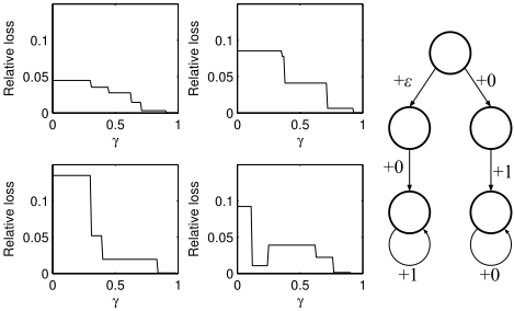
Our theoretical results translate various structural properties of an MDP onto a smooth upper-bound on the loss due to shallow planning. But what does the actual loss look like in any particular MDP? We know that the loss curve as a function of γ should be piecewise constant. This is because as we lower γ from γeval towards zero, there will be discrete points at which the optimal policy with respect to γ changes, partitioning the discount-factor interval and yielding a piecewise constant loss curve. This behavior of the loss curve is consistent with Blackwell optimality [Hordijk and Yushkevich, 2002], which asserts that at the extreme end near γ = 1 the loss curve is constant with value 0. This is seen in the 4 panels of Figure 2 where we plot the loss as a function of γ (see caption for additional details; we describe how the specific MDPs were generated below). What is perhaps interesting is that the loss curves are not always non-decreasing with increasing γ. The loss-curve in the bottom-right panel is clearly non-monotonic. The graph on the right of Figure 2 shows a simple MDP where it is easy to see how the loss can be nonmonotonic as a function of γ. Thus, loss-curves as a function of γ in any specific MDP can be complex and hard to predict using only high-level structural properties.

A useful way to illustrate the empirical validity of our monotonic theoretical results is to consider "average" loss curves by sampling MDPs from some distribution. Intuitively averaging multiple piecewise constant loss curves from perturbed MDPs should yield smooth loss curves (this is a form of smoothed analysis [Spielman and Teng, 2009]). Specifically, the results presented below will be of the following form. We will sample MDPs from multiple different generative-distributions defined in Section 5.1. Using procedures defined in Section 5.2, for each random MDP, we will compute the empirical value of the loss and the structural properties defined in Section 3.2 and 4. Then to show that the structural properties matter, we group their values into quantiles and plot an average loss curve for each quantile by averaging the loss curves over the MDPs that fall into that quantile. As we discuss below, we get the qualitative phenomenon expected from our theoretical results.

5.1 Domains Specification

We consider random MDPs with N states and 2 actions, generated according to the following schemes.

1. Random topologies: Each state-action pair is randomly assigned d possible next-states, where d is chosen according to one of the following:

fixed(N,d): d is a fixed number. binom(N,p): d is binomially distributed as B(N↪ p).

1. Ring topology ring(N,p): the N states form a ring. Upon taking action 1 at a state, the agent either stays at the same place or moves to the next state in clockwise order; the same for action 2 except that the agent moves in a counter-clockwise order. In addition, for each (s↪ a↪ s0 ) where s is not next to s0 , with probability p we add s0 as a next-state for (s↪ a).

Once the connectivity-structure of an MDP is determined as above, we fill the non-zero entries in the transition probabilities and the rewards with numbers drawn independently from U[0↪ 1] and normalize the transition probabilities.

5.2 Computing Structural Parameters

We compute the quantities that our theoretical results refer to for every randomMDP that we generate. Below is the list of quantities and how we compute them in practice:

1. Relative loss:

This is the empirical version of Equation 1, with a normalized magnitude between [0↪ 1].

1. Reward variation: we use ∆R◁maxs↪a R(s↪ a) as the empirical version of ∆R.
2. ✏-mixing time: we compute T⇡(✏) by its definition in Proposition 3 with ✏ = 0▷01↪ ⇡ = ⇡⇤ γeval . An implementation detail is that, we only search 50 steps for T⇡(✏) instead of checking an infinite number of steps, which is sufficient for the MDP distributions we consider in this paper. Formally, the empirical version of T⇡(✏) is inf {T  50 : 8s 2 S↪ T  t  50↪ ∥∥e>s [P ⇡ ]t - (⇢⇡ )>∥∥1  ✏ .
3. Stochastic diameter: to avoid the difficulty of calculating the stochastic distance between every pair of (s↪ s0 ), we compute its approximation by solving for the optimal value of an MDP Ms0 for each s0 instead: Ms0 has the same transition function as M except that s0 goes to an additional absorbing state s00 ; there is +1 reward when transitioning into s00 , and 0 everywhere else. Our empirical version of TM is then maxs↪s0 logγ V ⇡⇤Ms0 ↪γ Ms0 ↪γ (s) with γ = 0▷9999 (in fact, as γ tends to 1, this is equal to TM in the limit under mild conditions).
4. ✏-return mixing time: same as ✏-mixing time (✏ = 0▷01, checking for 50 steps).
5. Action Variation: we first compute for each s 2 S maxa↪a02A kP(·♣s↪ a) - P(·♣s↪ a0 )k1 in the definition of δP . Instead of taking max over all s, we take the average to be our empirical version of δP .

5.3 Results

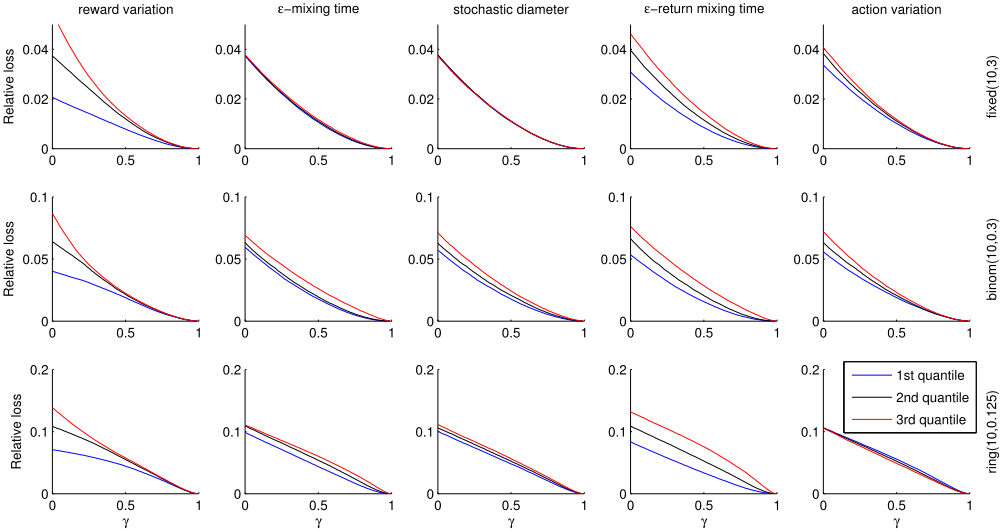
We present results for each of the following MDP distributions: fixed(10,3), binom(10,0.3), and ring(10,0.125). For each of the 5 structural parameters we have identified, we divide the 105 MDPs sampled from each distribution into 3 quantiles, and plot the relative loss averaged over each quantile of MDPs in Figure 3, where rows correspond to MDP distributions and columns correspond to identified parameters.Throughout the experiments we use γeval = 0▷995 and γ = 0↪ 0▷01↪ ▷ ▷ ▷ ↪ 0▷99.

As seen in Figure 3, although the loss for individual MDPs are piecewise constant curves and can have complicated shapes (see Figure 2), when averaged over a distribution over MDPs we get smooth loss curves monotonically decreasing with γ. Secondly, for each parameter, the loss curves for different quantiles are separated and exhibit the order predicted by our theoretical results (except in a few cases where the separation is not significant): all our bounds are monotonically increasing with the parameters, and in the results we see the loss curves corresponding to higher quantiles stay above those for lower quantiles, which validates our theoretical results.

6 RelatedWork

The simple bound obtained by combining Theorem 1 and Proposition 1 is very similar to that given by Kearns et al. [2002] where a discrete horizon is used instead of a continuous discount factor, and similar results have been implied in the convergence of value iteration [Sutton and Barto, 1998]. When planning with an inaccurate model under the problem specified horizon, the dependence of loss on planning horizon is well understood, especially when the model inaccuracy is due to statistical estimation errors [Mannor et al., 2007; Maillard et al., 2014] or approximation errors due to the use of function approximators [Ravindran and Barto, 2004; Taylor et al., 2009; Farahmand et al., 2010], or the combination of the two [Paduraru et al., 2008; Jiang et al., 2015a].

The papers mentioned above do not address the setting where γ < γeval, and as far as we know, Petrik & Scherrer [2009] were the first to examine this setting in the particular scenario where approximation schemes are deployed in dynamic programming. More recently, Jiang et al. [2015b] studied the impact of γ < γeval in another important scenario where there exists statistical estimation error in the model. In both these papers, the focus is on how the (negative) impact of model error grows as γ increases; to obtain the best policy via planning, such an impact has to be traded-off with the loss incurred by using γ when planning with a perfect model. Characterizing such a loss using structural properties of the MDP is exactly the topic of our paper, and we believe our study complements that of Petrik & Scherrer and Jiang et al., and provides a more complete picture of planning with smaller than specified horizons.

The structural parameters identified in this paper are inspired by some existing work: the notion of mixing times is often used in average time reward MDPs, e.g., [Kearns and Singh, 2002; Brafman and Tennenholtz, 2003], and a term similar to our definition of stochastic diameter is defined by Tewari and Bartlett [2008]. As far as we know, the other two parameters (reward variation and action variation), as well as the application of all of these parameters to bounding planning loss of shallow planning, are novel.

7 Conclusions

In this paper we presented multiple structural properties of MDPs that upper-bound the loss due to shallow planning with accurate models. Empirical results validated the role of these properties using a form of smoothed analysis.

Our theoretical results are also relevant to the setting of planning with inaccurate models learned from data as follows. As shown in Jiang et al. [2015b] an upper bound on the loss due to shallow planning with inaccurate models can be decomposed into two terms, an estimation error term that captures the loss due to the limited amount of data used to learn the model, and an approximation error term that captures the loss due to shallow planning. Our theoretical results can be viewed as providing structural parameters that affect the approximation error term.

Finally, our work provides the theoretical foundation for developing MDP planning algorithms that automatically choose an appropriate horizon. In fact, direct corollaries of our theory already offer some guidance on how to make such a choice: for example, if we have planned with a relatively small γ, the variation of the resulting value function (which is γ) provides a loss bound via Theorem 2. If the loss is affordable, we can choose not to re-plan with a larger γ in order to save computation. There is more work to be done towards a practical algorithm, and we leave this possibility for future exploration.

Acknowledgement

This work was supported by NSF grants IIS 1319365 (for Jiang and Singh) and IIS 1452099 (for Tewari). Any opinions, findings, conclusions, or recommendations expressed here are those of the authors and do not necessarily reflect the views of the sponsors.