
Adversarial Sequence Tagging
Proceedings of the Twenty-Fifth International Joint Conference on Artificial Intelligence. Pages 1690-1695.
Abstract
Providing sequence tagging that minimize Hamming loss is a challenging, but important, task. Directly minimizing this loss over a training sample is generally an NP-hard problem. Instead, existing sequence tagging methods minimize a convex upper bound that upper bounds the Hamming loss. Unfortunately, this often either leads to inconsistent predictors (e.g., max-margin methods) or predictions that are mismatched on the Hamming loss (e.g., conditional random fields). We present adversarial sequence tagging, a consistent structured prediction framework for minimizing Hamming loss by pessimistically viewing uncertainty. Our approach pessimistically approximates the training data, yielding an adversarial game between the sequence tag predictor and the sequence labeler. We demonstrate the benefits of the approach on activity recognition and information extraction/segmentation tasks.
- [Asif et al., 2015] Kaiser Asif, Wei Xing, Sima Behpour, and Brian D. Ziebart. Adversarial cost-sensitive classification. In Proceedings of the Conference on Uncertainty in Artifi- cial Intelligence, 2015.
- [Biggio et al., 2010] Battista Biggio, Giorgio Fumera, and Fabio Roli. Multiple classifier systems for robust classifier design in adversarial environments. International Journal of Machine Learning and Cybernetics, 1(1-4):27-41, 2010.
- [Crofoot et al., 2015] Margaret C Crofoot, Roland W Kays, and Martin Wikelski. Data from: Shared decision-making drives collective movement in wild baboons, 2015.
- [Dalvi et al., 2004] Nilesh Dalvi, Pedro Domingos, Sumit Sanghai, Deepak Verma, et al. Adversarial classification. In KDD, pages 99-108. ACM, 2004.
- [Grünwald and Dawid, 2004] Peter D. Grünwald and A. Phillip Dawid. Game theory, maximum entropy, min- imum discrepancy, and robust Bayesian decision theory. Annals of Statistics, 32:1367-1433, 2004.
- [Gurobi Optimization, 2015] Inc. Gurobi Optimization. Gurobi optimizer reference manual, 2015.
- [Hoffgen et al., 1995] Klaus-Uwe Hoffgen, Hans-Ulrich Si- mon, and Kevin S Vanhorn. Robust trainability of sin- gle neurons. Journal of Computer and System Sciences, 50(1):114-125, 1995.
- [Joachims et al., 2009] Thorsten Joachims, Thomas Finley, and Chun-Nam John Yu. Cutting-plane training of struc- tural SVMs. Machine Learning, 77(1):27-59, 2009.
- [Joachims, 1999] Thorsten Joachims. Making large scale SVM learning practical. Technical report, Universität Dort- mund, 1999.
- [Lafferty et al., 2001] John Lafferty, Andrew McCallum, and Fernando Pereira. Conditional random fields: Probabilis- tic models for segmenting and labeling sequence data. In Proc. of the International Conference on Machine Learn- ing, pages 282-289, 2001.
- [Lanckriet et al., 2003] Gert R.G. Lanckriet, Laurent El Ghaoui, Chiranjib Bhattacharyya, and Michael I. Jordan. A robust minimax approach to classification. JMLR, 3:555- 582, 2003.
- [Liao et al., 2007] Lin Liao, Dieter Fox, and Henry Kautz. Extracting places and activities from gps traces using hierar- chical conditional random fields. The International Journal of Robotics Research, 26(1):119-134, 2007.
- [Liu and Ziebart, 2014] Anqi Liu and Brian D. Ziebart. Ro- bust classification under sample selection bias. In Advances in Neural Information Processing Systems, 2014.
- [Liu, 2007] Yufeng Liu. Fisher consistency of multicategory support vector machines. In International Conference on Artificial Intelligence and Statistics, pages 291-298, 2007.
- [Lowd and Meek, 2005] Daniel Lowd and Christopher Meek. Adversarial learning. In Proceedings of the eleventh ACM SIGKDD international conference on Knowledge discovery in data mining, pages 641-647. ACM, 2005.
- [McCallum et al., 2000] A. McCallum, D. Freitag, and F. Pereira. Maximum entropy Markov models for infor- mation extraction and segmentation. In Proc. International Conference on Machine Learning, pages 591-598, 2000.
- [McMahan et al., 2003] H Brendan McMahan, Geoffrey J Gordon, and Avrim Blum. Planning in the presence of cost functions controlled by an adversary. In Proceedings of the International Conference on Machine Learning, pages 536- 543, 2003.
- [Reyes-Ortiz et al., 2015] Jorge-L Reyes-Ortiz, Luca Oneto, Albert Samà, Xavier Parra, and Davide Anguita. Transition- aware human activity recognition using smartphones. Neu- rocomputing, 2015.
- [Sarawagi and Cohen, 2004] Sunita Sarawagi and William W Cohen. Semi-markov conditional random fields for infor- mation extraction. In Advances in Neural Information Pro- cessing Systems, pages 1185-1192, 2004.
- [Sha and Pereira, 2003] F. Sha and F. Pereira. Shallow pars- ing with conditional random fields. In Proceedings of the Conference of the North American Chapter of the Associ- ation for Computational Linguistics on Human Language Technology, pages 134-141, 2003.
- [Strandburg-Peshkin et al., 2015] Ariana Strandburg- Peshkin, Damien R Farine, Iain D Couzin, and Margaret C Crofoot. Shared decision-making drives collective move- ment in wild baboons. Science, 348(6241):1358-1361, 2015.
- [Taskar et al., 2004] Ben Taskar, Carlos Guestrin, and Daphne Koller. Max-margin Markov networks. Advances in neural information processing systems, 16:25, 2004.
- [Topsøe, 1979] Flemming Topsøe. Information theoretical optimization techniques. Kybernetika, 15(1):8-27, 1979.
- [Tsochantaridis et al., 2004] Ioannis Tsochantaridis, Thomas Hofmann, Thorsten Joachims, and Yasemin Altun. Support vector machine learning for interdependent and structured output spaces. In Proceedings of the twenty-first interna- tional conference on Machine learning, page 104. ACM, 2004.
- [Vail et al., 2007] Douglas L. Vail, Manuela M. Veloso, and John D. Lafferty. Conditional random fields for activ- ity recognition. In Proc. International Conference on Autonomous Systems and Multiagent Systems, pages 1-8, 2007.
- Viterbi, 1967
- Andrew J Viterbi. Error bounds for convo- lutional codes and an asymptotically optimum decoding algorithm. Information Theory, IEEE Transactions on, 13(2):260-269, 1967.
- [von Neumann and Morgenstern, 1947] John von Neumann and Oskar Morgenstern. Theory of Games and Economic Behavior. Princeton University Press, 1947.
- [Wang et al., 2015] Hong Wang, Wei Xing, Kaiser Asif, and Brian D. Ziebart. Adversarial prediction games for multi- variate losses. In Advances in Neural Information Process- ing Systems, 2015.
References were extracted automatically from the PDF and may contain errors.
Full text extracted automatically from the PDF; figures, tables and equations may differ. The PDF is the version of record.
1 Introduction
Sequence tagging methods that jointly predict interdependent variables are needed in applications ranging from natural language processing [Lafferty et al., 2001; Sha and Pereira, 2003] to activity recognition [Vail et al., 2007; Liao et al., 2007]. Unfortunately, obtaining a parametric predictor that directly minimizes the Hamming loss (the number of incorrectly predicted variables) is an NP-hard empirical risk minimization (ERM) problem [Hoffgen et al., 1995] in general. Conditional random fields [Lafferty et al., 2001] and maximum margin methods (e.g., structural support vector machines [Joachims et al., 2009] and maximum margin Markov networks [Taskar et al., 2004]) instead minimize convex surrogates of the Hamming loss (i.e., the logarithmic loss and the hinge loss). This mismatch between the surrogate loss function and the Hamming loss leads to inconsistency and sub-optimal predictive performance.
We present adversarial sequence tagging (AST), a supervised sequence tagging approach that is both consistent for the Hamming loss and provides good predictive performance in practice by adversarially approximating the training data. At its core, our approach reduces prediction to solving a zerosum game based on the Hamming loss between a prediction player trying to minimize the loss and an adversarial player trying to maximize it while being constrained to reflect properties of the training data. Parameter estimation is solved as a convex optimization problem under this formulation even though minimizing the Hamming loss is non-convex in ERM formulations. Our contributions in this paper are:
⇤Both authors contributed equally.
- We extend adversarial loss minimization methods for classification [Asif et al., 2015] and multivariate performance measures [Wang et al., 2015] to the structured prediction setting of sequence tagging.
- We establish the Fisher consistency of our adversarial prediction method and contrast it with the inconsistency of maximum margin methods for sequence prediction.
- We scale our approach to long sequences of variables with many possible values by leveraging an independence property that allows a single oracle inference method (in contrast, double oracle is exclusively required for multivariate losses [Wang et al., 2015]).
- We evaluate our approach on natural language processing and activity recognition tasks, demonstrating its competitive predictive performance compared with maximum margin methods and CRFs.
2 Background and RelatedWork
2.1 Notation
In this work, we seek a sequence predictor, ˆ P(y♣x), for variables y = y1:T = ¶y1↪ y2↪ ▷ ▷ ▷ ↪ yT ♦ 2 Y, conditioned on provided input variables, x = x1:T = ¶x1↪ x2↪ ▷ ▷ ▷ ↪ xT♦ 2 X. We consider the supervised learning setting where m sequence examples, ¶y(j) ↪ x(j) ♦j=1:m drawn from empirical training distribution ˜ P(x↪ y) (samples from true distribution P(y↪ x)), are available to estimate the model. We distinguish between the actual label variables, y, and the predicted label variables, ˆy, using "hat" notation, and will later introduce a set of adversarially-chosen labels ˇy = ¶ˇ y1↪ ˇ y2↪ ▷ ▷ ▷ ↪ ˇ yT♦. We make extensive use of expectation notation, EP(x)[f(X)] = Px2X P(x)f(x), in which random variables are capitalized. We also denote statistics of the sequence of variables as
Φ(x↪ y) 2 Rk . These typically decompose additively over the sequence: e.g., Φ(x↪ y) = PT-1 t=1 φ(x↪ yt:t+1).
2.2 Empirical Sequence RiskMinimization
Conditional random fields (CRFs) and structured support vector machines (SSVMs) are two prominent methods for sequence tagging based on minimizing the empirical risk:
For conditional random fields [Lafferty et al., 2001], the logarithmic loss, -log ˆ P(y♣x), and an exponential random field model, e.g., ˆ P(y♣x) / exp(✓ · Φ(x↪ y)) are employed in Eq. (1). For structured support vector machines [Tsochantaridis et al., 2004], the structured hinge loss is a convex approximation to the Hamming loss, ∆(y↪ ˆy) = PTt=1 I(ˆ yt 6= ˜ yt),
where [f(x)]+ , max(0↪ f(x)), and a linear discriminant function, ˆ f✓(x) = argmaxˆy2Y ✓ · Φ(x↪ ˆy), are employed in Eq. (2). The loss function of each model is a convex upper bound on the Hamming loss, PTt=1 I(ˆ yt 6= ˜ yt).
2.3 Sequence Tagging Consistency
Predictors that minimize a loss measure when provided with the true data distribution for training are desirable. Definition 1 formalizes this notion in terms of the Fisher consistency.
Definition 1. Predictor ˆ f(x) with full representational ability (e.g., parameterized by potential functions (x↪ y)) is Fisher consistent for loss function ∆(ˆf(x)↪ y) if it minimizes the expected loss, EP(x↪y)[∆( ˆ f(X)↪Y)], when trained (e.g., surrogate ERM) under the true data distribution P(x↪ y).
Similar to multi-class SVM incosistency [Liu, 2007], Theorem 1 shows SSVM's inconsistency for sequence tagging. This inconsistency motivates our desires for a better method.
Theorem 1. Given the distribution P11 = 0▷4, P22 = 0▷3, P33 = 0▷3, and Pij = 0 8i 6= j over sequences of length two, where Pij compactly denotes P(y1 = i↪ y2 = j♣x), the hinge loss of SSVM is not Fisher consistent for the Hamming loss.
Proof. For SSVM and Hamming loss, ⇤ minimizes:
The minimizer ⇤ must satisfy (x↪ 11) ≥ (x↪ y0 ) where y0 6= 11. Otherwise, the result will not be Fisher consistent. Assume (w.l.o.g.) (x↪ 22) ≥ (x↪ 33). (4) becomes P11 [maxy0 6=11¶∆(11↪ y0 ) + (x↪ y0 ) - (x↪ 11)♦]+ + 0 + 0 +0+P22 [maxy0 6=22¶∆(22↪ y0 ) + (x↪ y0 ) - (x↪ 22)♦]+ +0 + 0 + 0 + P33[maxy0 6=33¶∆(33↪ y0 ) + (x↪ y0 )
- (x↪ 33)♦]+. Since (x↪ 11) ≥ (x↪ y0 ), (x↪ 11) - (x↪ 22) > (x↪ y0 ) - (x↪ 22), for y0 6= 11, 2 is the maximum Hamming loss for length 2 sequences. As a result, [maxy0 6=22¶∆(22↪ y0 ) + (x↪ y0 ) - (x↪ 22)♦]+ = 2+ (x↪ 11) - (x↪ 22). Similarity, [maxy0 6=33¶∆(33↪ y0 ) + (x↪ y0 )- (x↪ 33)♦]+ = 2+ (x↪ 11)- (x↪ 33). The expected hinge loss is P11[maxy0 6=11¶∆(11↪ y0 ) + (x↪ y0 ) - (x↪ 11)♦]+ + P22(2 + (x↪ 11) - (x↪ 22)) + P33(2 + (x↪ 11) - (x↪ 33)). When (x↪ 11) = (x↪ 22) = (x↪ 33) ≥ (x↪ ij)↪ 8i 6= j, the loss is 2. For any other case [maxy0 6=11¶∆(11↪ y0 ) + (x↪ y0 ) - (x↪ 11)♦]+ , we show the loss exceeds 2:
Case 1: whenmaxy0 6=11¶∆(11↪ y0 )+ (x↪ y0 )- (x↪ 11)♦ 0, then 2+ (x↪ 22)- (x↪ 11) < 0, (x↪ 11)- (x↪ 22) ≥ 2. Similarly, (x↪ 11) - (x↪ 33) ≥ 2. The loss is P22(2 + (x↪ 11)- (x↪ 22))+P33(2+ (x↪ 11)- (x↪ 33)) ≥ 4(P22+ P33). As long as P22 +P33 > 0▷5, this is greater than 2. Case 2: whenmaxy0 6=11¶∆(11↪ y0 )+ (x↪ y0 - (x↪ 11)♦ > 0, we have maxy0 6=11 ¶∆(11↪ y0 ) + (x↪ y0 ) - (x↪ 11)♦ ≥ 2+ (x↪ 22)- (x↪ 11). We also have (x↪ 11)- (x↪ 33) ≥ (x↪ 11) - (x↪ 22) The loss is at least P11(2 + (x↪ 22) - (x↪ 11))+P22(2+ (x↪ 11)- (x↪ 22))+P33(2+ (x↪ 11)- (x↪ 33)) ≥ 2(P11+P22+P33)+P11( (x↪ 22)- (x↪ 11))+ P22( (x↪ 11)- (x↪ 22))+P33( (x↪ 11)- (x↪ 22)). When P22 + P33 > 0▷5, the loss exceeds 2. We can see that in the example, the minimized value for the loss function is 2 and is achieved when (x↪ 11) = (x↪ 22) = (x↪ 33). Since argmax cannot distinguish between the different labels, SSVM is not Fisher consistent.
2.4 Adversarial Estimation
We expand upon prior perspectives for prediction as an adversarial task [Dalvi et al., 2004; Lowd and Meek, 2005; Biggio et al., 2010]. However, unlike those works, we do not assume that the data comes from an adversary attempting to corrupt the test data to, e.g., defeat a spam filter. Instead, our approach is more closely related to the duality between worst-case minimization of information-theoretic loss functions and maximum likelihood estimation of exponential family member probability distributions [Topsøe, 1979; Gr¨unwald and Dawid, 2004; Liu and Ziebart, 2014] and methods that parametrically constrain the adversary [Lanckriet et al., 2003].
Our method follows two recent advances in adversarial classification: a general formulation of cost-sensitive classification as a zero-sum prediction game [Asif et al., 2015]; and adversarial prediction games for multivariate performance measures [Wang et al., 2015]. These previous methods for univariate predictions do not incorporate correlative relationships between predicted variables and cannot be effectively employed for sequence tagging tasks. We demonstrate how the adversarial formulation can be extended to the structured prediction setting using constraint generation methods known as the single and double oracle [McMahan et al., 2003] to avoid exponentially-sized zero-sum games from the latter work [Wang et al., 2015] in the sequence tagging setting. The key difference is that feature functions are multivariate in this work, while loss functions are multivariate in that prior work.
3 Adversarial Sequence Tagging Games
Motivated by the mismatch between convex surrogates and loss measures of interest, we develop our adversarial approach for sequence tagging.
3.1 Adversarial Formulation
Instead of choosing a predictor's parametric form and using ERM on training data to select its parameters, we obtain the predictor that performs best for the worst-case choice of conditional label distributions that match statistics measured from available training data. As we shall see, sequence loss functions for which empirical risk minimization is nonconvex and NP-hard can often be solved efficiently in this formulation.
Following recently developed methods for adversarial costsensitive classification [Asif et al., 2015], we pose structured prediction as an adversarial game in which an estimator player chooses a conditional distribution, ˆ P(ˆy♣x). An adversarial player then chooses a distribution, ˇ P(ˇy♣x), from the set of distributions matching certain statistics, Φ(x↪ y). The estimator player seeks to minimize an expected loss, while the adversary seeks to maximize this loss:
where the feature functions, Φ(x↪ y), typically additively decompose over pairs of the Y1↪ ▷ ▷ ▷ ↪ YT variables: e.g., Φ(x↪ y) = PT-1 t=1 φ(x↪ yt↪ yt+1).
By leveraging Lagrangian and zero-sum game duality, this formulation reduces to a convex optimization problem:
where ˆpx and ˇpx are vector representations of the conditional label distributions, P(ˆy♣x) and P(ˇy♣x) and C0x↪✓ is a payoff matrix that incorporates both the loss function and a Lagrangian potential term that enforces the optimization's constraints: (C0x↪y↪✓ )ˆy↪ˇy = loss(ˆy↪ ˇy) + ✓ · (φ(x↪ ˇy) - φ(x↪ y)). Table 1 is the payoff matrix of the 3-length binary-valued sequence game. Rows represent the predictor's pure strategies. Columns represent the adversary's pure strategies. Each payoff combines the Hamming loss (e.g., 1 for sequences 001 and 101) and a Lagrangian potential motivating the adversary to behave "similarly to" training data.
Zero-sum games can be solved as linear programs to find each player's mixed Nash equilibrium [von Neumann and Morgenstern, 1947]. For example, the mixed Nash equilibrium strategy for the adversarial player is obtained from:
Similarly, the predictor's mixed Nash equilibrium strategy is:
These sets of inequality constraints ensure the game value v is constrained by all possible pure strategies of the opponent.
| 000 | 001 | 010 | 011 | 100 | 101 | 110 | 111 | |
|---|---|---|---|---|---|---|---|---|
| 0+ 000 | 1+ 001 | 1+ 010 | 2+ 011 | 1+ 100 | 2+ 101 | 2+ 110 | 3+ 111 | 000 |
| 1+ 000 | 0+ 001 | 2+ 010 | 1+ 011 | 2+ 100 | 1+ 101 | 3+ 110 | 2+ 111 | 001 |
| 1+ 000 | 2+ 001 | 0+ 010 | 1+ 011 | 2+ 100 | 3+ 101 | 1+ 110 | 2+ 111 | 010 |
| 2+ 000 | 1+ 001 | 1+ 010 | 0+ 011 | 3+ 100 | 2+ 101 | 2+ 110 | 1+ 111 | 011 |
| 1+ 000 | 2+ 001 | 2+ 010 | 3+ 011 | 0+ 100 | 1+ 101 | 1+ | 110 2+ 111 | 100 |
| 2+ 000 | 1+ 001 | 3+ 010 | 2+ 011 | 1+ 100 | 0+ | 101 | 2+ 110 1+ 111 | 101 |
| 2+ 000 | 3+ 001 | 1+ 010 | 2+ | 011 1+ | 100 | 2+ 101 | 0+ 110 | 110 1+ 111 |
| 3+ 000 | 2+ 001 | 2+ | 010 | 1+ 011 | 2+ 100 | 1+ 101 | 1+ 110 | 111 0+ 111 |
Extending adversarial classification [Asif et al., 2015] to sequence tagging settings leads to inner zero-sum matrix games characterized by C0x↪✓ with ♣Y♣T value assignment "pure strategies" for each player. As a consequence, explicitly constructing the corresponding game matrix is intractable for all but the smallest of sequence tagging tasks.
3.2 Double Oracle Method for Efficient Prediction
We overcome the computational difficulties of constructing the entire adversarial game using the double oracle algorithm [McMahan et al., 2003] to iteratively construct an appropriate reduced game that still provides the correct equilibrium. This approach was previously applied to obtain game solutions for multivariate performance measures [Wang et al., 2015]. We extend this to structured prediction problems where consecutive variables are related by measured statistics.
The double oracle game solver considers a subset of pure strategies, ˆ S or ˇ S, for each player. It constructs the payoff matrix and obtains the mixed Nash equilibrium for this subset of pure strategies. It then finds the best response pure strategy, ˇyBR or ˆyBR, for the player in response to the opponent's equilibrium mixed strategy, ˆ P(ˆy♣x) or ˆ P(ˇy♣x), and adds it to the set of pure strategies. The algorithm terminates when neither player can improve upon their strategy with additional actions. Thus, the strategies it returns are a Nash equilibrium pair [McMahan et al., 2003]. We refer interested readers to Wang et. al [Wang et al., 2015] for more details. The major difference for sequence tagging from that previous work is in finding best responses. We find the best response ˇyBR pure strategy to add to the game according to the maximization of:
which is recursively defined from marginal probabilities ˆ P (ˆ yi) as shown, and solved using the Viterbi algorithm
[Viterbi, 1967] by iteratively computing for t = ¶T↪ · · · ↪ 1♦: β(ˇ yt) = Eˆ P (ˆ yt) hI( ˆ Yt 6= ˇ yt)i + maxˇ yt+1 ✓ · φ(x↪ ˇyt:t+1) + β(ˇ yt+1) and storing the maximizing variable assignment.
For the complementary problem of adding the best ˆy action to the game, we choose ˆy according to: argminˆy Eˇ p(ˇy♣x) [loss(ˆy↪ ˇy)]. For the Hamming loss, each term of the best response sequence can be independently obtained from ˆyBR = ¶argmaxyt ˇ P (yt♣x)♦Tt=1 .
3.3 Single Oracle Method for Efficient Prediction
So long as the loss function additively decomposes into payoff matrix terms Ct for each t 2 ¶1↪ ▷ ▷ ▷ ↪ T♦, the estimator's predictions are independent (as observed when finding the best response for the double oracle method). This is in contrast with adversarial prediction methods for structured losses [Wang et al., 2015], in which the loss function prevents independence from both adversary and predictor. The independence found in the sequence tagging game allows the combination of all estimator's "pure strategies" in the sequence tagging game to be efficiently considered using the following pair of linear programs:
As the entire set of predictor pure strategies is considered by this revised set of linear programs, the double oracle method can be reduced to a single oracle method. Only the adversary's set of pure strategies over the entire sequence needs to be expanded in this approach (Algorithm 1).
Algorithm 1 Single Oracle Game Solver
Input: Lagrangian potential, ; initial action set ˇ S Output: [ ˆ P(ˆy♣x)↪ ˇ P (ˇy♣x)] ˇyBR ¶♦ repeat Ct buildPayoffMatrices( ˇ S, ) [ ˆ P(ˆy♣x), vNash1 ] solveZeroSumGameˆ Y (C) [ˇyBR, ˇ vBR] findBestResponseStrategy( ˆ P(ˆy♣x), ) ˇ S ˇ S [ ˇyBR until (vNash1 = ˇ vBR) return [ ˆ P(ˆy♣x), ˇ P (ˇy♣x)]The size of the payoff matrix, C' from Eq. (7), in the double oracle method is O(♣ ˆ S♣♣ ˇ S♣), while the single oracle method corresponds to a matrix of size O(♣ ˇ S♣T♣Y♣). Computational benefits may thus be realized by this approach when the number of estimator pure strategies in the double oracle method is sufficiently large. In such cases, reducing the overall size of the payoff matrix compensates for the added complexity of the linear program in the single oracle method. In
Algorithm 2 Parameter Estimation Algorithm
Input: Training dataset D with pairs (x↪ y) 2 D, feature
function Φ : X [ Y ! Rk , learning rate ¶γt♦ Output: Model parameter estimate ✓ t 1 while ✓ not converged do Random shuffle samples for stochastic training for all (x↪ ˜y) 2 D do Compute ˇ P(ˇy♣x) using single/double oracle r✓ EˇP(y♣x) [Φ(x↪ ˇy)] -Φ(x↪ ˜y) ✓ ✓ -γtr✓; t t + 1 end for end while
practice, a hybrid approach that switches between single oracle and double oracle methods based on the length of the sequence can be used to yield faster predictions.
3.4 Learning via Convex Optimization
We employ stochastic gradient descent to obtain the AST model parameters. As described in Algorithm 2, for each iteration in the update, we use single oracle (Algorithm 1) or double oracle to find the adversary's Nash equilibrium solution to the AST game: ˇ P(ˇy♣x). Feature expectations are calculated according to Eq. (12):
This feature expectation under the adversary's distribution is then used to calculate the gradient, as shown in Algorithm 2. Due to convexity, this optimization procedure converges to a global optima given appropriate learning rate parameters γt.
3.5 Consistency
An important benefit of AST over maximum margin methods is the consistency guarantee it provides.
Theorem 2. Given that the sequence's probability distribution factors according to the chain independence assumptions: P(y♣x) = QTt=1 P(yt♣yt-1↪ x1:T ), and an arbitrarily rich feature representation, (yt↪ yt+1↪ x1:T ), the AST method provides the loss-optimal sequence tagging, argminˆy EP(Y♣x) [loss(ˆy↪Y)].
Proof. The Lagrangian of Eq. (6) gives, equivalently:
where: (a) follows from Lagrangian duality and rearranging the expectation terms; Eq. (14) can only avoid being unboundedly negative by choosing ˇ P(y♣x) = P(y♣x), leading to cancellations of (b) 1 ; and reducing the minimization of a linear function to a non-probabilistic decision via (c). This is, by definition, the set of risk-minimizing predictions.
Thus, when learning from any true distribution of sequence data, P(y↪ x), using a sufficiently expressive feature representation to capture its sequential relationships, the predictor minimizing the Hamming loss will be obtained.
4 Experiments
In this section, we demonstrate the effectiveness of our proposed AST model.
4.1 Dataset Descriptions
We investigate activity recognition datasets (for both human or animal activities), and natural language processing datasets. The properties of the training datasets and testing datasets are summarized in Table 2.
| Name | Classes | Attributes | Train/Test Sequences | Train/Test Variables |
|---|---|---|---|---|
| Human Activity | 12 | 561 | 395 / 174 | 7767 / 3162 |
| Baboon (day 1) | 7 | 24 | 12 / 12 | 718 / 718 |
| Baboon (day 2) | 7 | 24 | 12 / 12 | 718 / 718 |
| FAQSeg | 4 | 24 | 26 / 22 | 36327 / 21618 |
Human Activity Recognition Dataset [Reyes-Ortiz et al., 2015] was collected from 30 volunteers wearing smart phones on their waists. There are 12 different activities labeled in this dataset (walking, walking upstairs, walking downstairs, sitting, standing, laying, stand-to-sit, sit-to-stand, sit-to-lie, lie-to-sit, stand-to-lie, and lie-to-stand). We segment the data into consecutive temporal sequences. There are 561 features for each time step based on accelerometer and gyroscope measurements collected from the smart phones.
1 For additively decomposing potentials, (x↪ y) = Pt 0 (x↪ yt↪ yt+1), only pairwise conditional probabilities must match: ˆ P(yt↪ yt+1♣x) = P(yt↪ yt+1♣x). However, since P(y♣x) is Markovian by assumption, the entire conditional sequence distributions match as well.
Baboon Activity Recognition Dataset [Strandburg-Peshkin et al., 2015; Crofoot et al., 2015] consists of GPS and accelerometer data gathered for 12 hours each day for 35 days from 26 adult and sub-adult members of a baboon troop wearing sensor collars. Four experts labeled two days of troop activities (e.g. sleeping, hanging out, coordinated progression, coordinated non-progression). We consider the majority vote of their annotations to be the ground truth label. We segment each day of data into 12 one hour sequences. We use 24 features to create each prediction model. These include the average speed of the group and other group location-based measurements. We report two results: using the labeled first day of data to classify the second day's activities (Baboon (day 1)); and using the second day's labeled data to classify the first day's activities (Baboon (day 2)).
FAQ Segmentation Dataset [McCallum et al., 2000] contains 48 Frequently Asked Questions (FAQs) downloaded from the Internet. 26 are used for training and 22 for testing. Each line in the document is labeled with four possible labels: head, question, answer, and tail. 24 Boolean features are generated for each line.
4.2 Methodology
We compare our proposed adversarial sequence tagging model against the state-of-the-art methods for structured prediction. The methods details are as follows:
A linear chain Conditional Random Field (CRF) [Sarawagi and Cohen, 2004] with features based on the transition between labels φ(yt↪ yt+1) and input variables/labels φ(xt↪ yt). We use LBFGS for optimizing the model. We selected the regularization weights using a validation set (approximately 10% of the data) 2 .
For Structural SVM (SSVM), we use the SVM hmm implementation of structural SVM inside the SVM light package [Joachims, 1999]. SVM hmm is implemented to learn a model with chain structure. We include the first-order tag sequence as features. We use a validation set of 10% of the data for selecting the parameter c which controls the trade-off between slack and the magnitude of the weights vectors, and default parameters for the remaining settings.
For our Adversarial Sequence Tagging (AST) approach, we implemented our previously described learning and prediction algorithms. Our features are those of the CRF package [Sarawagi and Cohen, 2004]. For training and testing, we use the oracle approach on each data sequence. We optimized using stochastic gradient descent to learn the AST model parameters. We note that the initial action set for our methods does not significantly influence the results (we use sequences ¶11 ▷ ▷ ▷ 1, 22 ▷ ▷ ▷ 2, ▷ ▷ ▷♦ for each player). We use deterministic predictions using the sequence with the maximum probability rather than making stochastic predictions. We use Gurobi [Gurobi Optimization, 2015] as the linear programming solver to compute equilibria.
2 Since the number of baboon data sequences is small, we did not use a validation set for parameter tuning in baboon experiments.
| Dataset | CRF | SSVM | AST |
|---|---|---|---|
| Human Activity | 97.12% | 97.03% | 97.19% |
| Baboon (day 1) | 75.63% | 75.63% | 77.30% |
| Baboon (day 2) | 68.66% | 63.65% | 69.22% |
| FAQSeg | 87.62% | 94.23% | 94.42% |
4.3 Results
We evaluate performance, shown in Table 3, using the pervariable accuracy (the complement of the Hamming loss) as our performance measure. Our proposed approach, AST, consistently outperforms the CRF and SSVM on the four datasets. However, SSVM performs sometimes better and sometimes worse than CRF. The reason is likely due to the convex approximation of the hinge loss and logloss, which can create more errors in some cases. In contrast, our approach, AST, outperforms CRF and SSVM by minimizing the loss for an adversarial approximation of the training data. This upper bounds the generalization loss since real data is not likely to be worst case. Other approaches minimize surrogate losses, which upper bound the Hamming loss, on training data samples. These two approaches can be viewed as approximating the training data (and using the exact loss function of interest) versus approximating the loss function (and using the exact training data). We believe the former more closely aligns with test performance. Our consistency results show this to be true for certain feature representations and data distributions when compared to the hinge loss surrogate of the Hamming loss.
The differences in loss measures that the methods attempt to optimize offers some explanation for the performance differences of CRF and SSVM. For example, the hinge loss approximation of the Hamming loss on test data for FAQSeg is 2,816.04 for SSVM, 3,961.25 for CRF, and 35,291.35 for AST. Thus, SSVM is providing much better performance on the measure it is designed to minimize, but this does not translate into better Hamming loss due to differences introduced by the hinge approximation.
| Dataset | CRF | SSVM | AST |
|---|---|---|---|
| Human Activity | 1050 | 0.04 | 193 |
| Baboon (day 1) | 4.8 | 0 | 2.6 |
| Baboon (day 2) | 4.5 | 0 | 2.5 |
| FAQSeg | 108 | 0.1 | 15.8 |
Table 4 shows the amount of time required to make predictions for all of the testing sequences. The SSVM package is well optimized so that the running time is very fast. This provides a good baseline for comparison. Although the AST model takes longer than the SSVM approach, the improvement in accuracy can often be worth the additional running time. At the same time, the AST model's computation time is in some cases almost an order of magnitude more efficient than CRF prediction, which is limited by the need to compute the normalization term for a distribution over sequences.
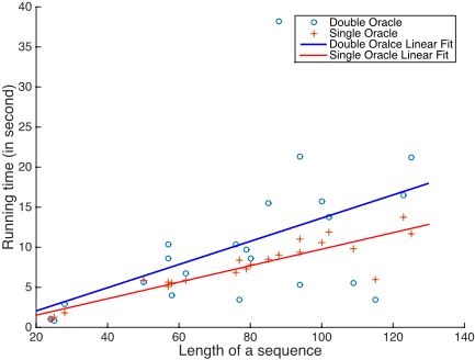
Figure 1 shows the running time comparing double oracle and single oracle approaches on the more time-consuming Human Activity dataset on test instances of minimum length 20. For longer sequences, single oracle requires less time than double oracle. This demonstrates that the single oracle can be useful for long sequences with many labels. Unfortunately, for very short sequences (e.g., those less than length 20), the double oracle method is consistently more efficient on average. When short sequences dominate the distribution of training data, which is the case for many problems, the single oracle method's average running time is slower than double oracle method. This suggests a hybrid approach that uses the double oracle method for short sequences and the single oracle method for longer sequences.
5 Conclusion
We have developed AST, a sequence tagging method for inductively minimizing Hamming loss that is both consistent and performs well in practice. This stands in contrast with existing methods: maximum margin methods (SSVMs and M3Ns) are not consistent and can be shown to have arbitrarily large loss for certain data distributions; conditional random fields, though consistent, use a surrogate loss that differs substantially from the Hamming loss. For both alternatives, we have shown AST to provide better sequence tags. Further, we have introduced a single oracle inference procedure for AST that improves the computational efficiency of the approach on tasks with long sequences and many possible labels.
Acknowledgments
The research in this paper was supported in part by the NSF grants III-1514126 (Ziebart, Berger-Wolf), CNS-1248080 (Berger-Wolf), and RI-1526379 (Ziebart). We thank the reviewers for their valuable comments.
@inproceedings{ijcai2016p242,
  title     = {Adversarial Sequence Tagging},
  author    = {Li, Jia and Asif, Kaiser and Wang, Hong and Ziebart, Brian D. and Berger-Wolf, Tanya Y.},
  booktitle = {Proceedings of the Twenty-Fifth International Joint Conference on
               Artificial Intelligence, {IJCAI-16}},
  publisher = {AAAI Press / International Joint Conferences on Artificial Intelligence},
  editor    = {Subbarao Kambhampati},
  pages     = {1690--1695},
  year      = {2016},
  month     = {7},
  url       = {https://ijcai.org/proceedings/2016/242},
}
TY - CPAPER TI - Adversarial Sequence Tagging AU - Li, Jia AU - Asif, Kaiser AU - Wang, Hong AU - Ziebart, Brian D. AU - Berger-Wolf, Tanya Y. T2 - Proceedings of the Twenty-Fifth International Joint Conference on Artificial Intelligence, IJCAI-16 PB - AAAI Press / International Joint Conferences on Artificial Intelligence PY - 2016 SP - 1690 EP - 1695 UR - https://ijcai.org/proceedings/2016/242 ER -Copied
Machine-readable versions of this paper, for tools and AI agents:





