
Multi-View Learning with Limited and Noisy Tagging
Proceedings of the Twenty-Fifth International Joint Conference on Artificial Intelligence. Pages 1718-1723.
Abstract
Multi-view tagging has become increasingly popular in the applications where data representations by multiple views exist. A robust multi-view tagging method must have the capability to meet the two challenging requirements: limited labeled training samples and noisy labeled training samples. In this paper, we investigate this challenging problem of learning with limited and noisy tagging and propose a discriminative model, called MSMC, that exploits both labeled and unlabeled data through a semi-parametric regularization and takes advantage of the multi-label space consistency into the optimization. While MSMC is a general method for learning with multi-view, limited, and noisy tagging, in the evaluations we focus on the specific application of noisy image tagging with limited labeled training samples on a benchmark dataset. Extensive evaluations in comparison with state-of-the-art literature demonstrate that MSMC outstands with a superior performance.
- [Barnard et al., 2003] Kobus Barnard, Pinar Duygulu, David Forsyth, Nando de Freitas, David M. Blei, and Michael I. Jordan. Matching words and pictures. Journal of Machine Learning Research, 3:1107-1135, 2003.
- [Blei and Jordan, 2003] David M. Blei and Michael I. Jor- dan. Modeling annotated data. In Proceedings of the 26th International ACM SIGIR Conference, 2003.
- [Bouboulis et al., 2010] Pantelis Bouboulis, Konstantinos Slavakis, and Sergios Theodoridis. Adaptive kernel- based image denoising employing semi-parametric reg- ularization. IEEE Transactions on Image Processing, 19(6):1465-1479, 2010.
- [Chua et al., 2009] Tat Seng Chua, Jinhui Tang, Richang Hong, Haojie Li, Zhiping Luo, and Yantao Zheng. Nus- wide: a real-world web image database from national uni- versity of singapore. In Proceedings of the ACM Inter- national Conference on Image and Video Retrieval, pages 1-9, 2009.
- [Farquhar et al., 2006] J. Farquhar, D. Hardoon, H. Meng, J. Shawe-Taylor, and S. Szedmak. Two view learning: SVM-2K, theory and practice. In Advances in Neural In- formation Processing Systems. MIT Press, 2006.
- [Gill and Wong, 2015] Philip E. Gill and Elizabeth Wong. Methods for convex and general quadratic programming. Math. Program. Comput., 7(1):71-112, 2015.
- [Goh et al., 2001] King-Shy Goh, Edward Chang, and Kwang-Ting Cheng. SVM binary classifier ensembles for image classification. In Proceedings of the tenth interna- tional conference on Information and knowledge manage- ment, pages 395-402, 2001.
- [Guo et al., 2008] Zhen Guo, Zhongfei (Mark) Zhang, Eric P. Xing, and Christos Faloutsos. Semi-supervised learning based on semiparametric regularization. In SDM, pages 132-142, 2008.
- [Li et al., 2010] Guangxia Li, Steven C. H. Hoi, and Kuiyu Chang. Two-view transductive support vector machines. In SDM, pages 235-244, 2010.
- [Li et al., 2013] Yingming Li, Zhongang Qi, Zhongfei (Mark) Zhang, and Ming Yang. Learning with limited and noisy tagging. In Proceedings of ACM MM, pages 957-966, 2013.
- [Lin and de Wang, 2004] Chun F. Lin and Sheng de Wang. Training algorithms for fuzzy support vector machines with noisy data. Pattern Recognition Letters, 25:1647- 1656, 2004.
- [Liu and Zheng, 2007] Yi Liu and Yuan F. Zheng. Soft SVM and its application in video-object extraction. IEEE Trans- actions on Signal Processing, 55(7-1):3272-3282, 2007.
- [Liu et al., 2010] Dong Liu, Xian-Sheng Hua, Meng Wang, and Hong-Jiang Zhang. Image retagging. In Proceedings of ACM MM, pages 491-500, 2010.
- [Liu et al., 2015] Meng Liu, Yong Luo, Dacheng Tao, Chao Xu, and Yonggang Wen. Low-rank multi-view learning in matrix completion for multi-label image classification. In AAAI, pages 2778-2784, 2015.
- [Qi and Han, 2007] Xiaojun Qi and Yutao Han. Incorporat- ing multiple SVMs for automatic image annotation. Pat- tern Recognition, 40:728-741, 2007.
- [Qi et al., 2012] Zhongang Qi, Ming Yang, Zhongfei (Mark) Zhang, and Zhengyou Zhang. Multi-view learning from imperfect tagging. In ACM Multimedia, pages 479-488, 2012.
- [Rosenberg et al., 2009] David S. Rosenberg, Vikas Sind- hwani, Peter L. Bartlett, and Partha Niyogi. A kernel for semi-supervised learning with multi-view point cloud reg- ularization. In IEEE Signal Processing Magazine, 2009.
- [Ruppert et al., 2003] David Ruppert, M. P. Wand, and R. J. Carroll. Semiparametric Regression. Cambridge Univer- sity Press, Cambridge, UK, 2003.
- [Schölkopf and Smola, 2001] Bernhard Schölkopf and Alexander J Smola. Learning with Kernels: Support Vector Machines, Regularization, Optimization, and Beyond. The MIT Press, 2001.
- [Schölkopf et al., 1997] Bernhard Schölkopf, Alex J. Smola, and Klaus-Robert Müller. Kernel principal component analysis. In ICANN, pages 583-588, 1997.
- [Sindhwani and Rosenberg, 2008] Vikas Sindhwani and David S. Rosenberg. An rkhs for multi-view learning and manifold co-regularization. In ICML, pages 976-983, 2008.
- [Smola et al., 1998] Alexander J. Smola, Thilo-Thomas Frieß, and Bernhard Schölkopf. Semiparametric support vector and linear programming machines. In NIPS, pages 585-591, 1998.
- [Tang et al., 2011] Jinhui Tang, Richang Hong, Shuicheng Yan, Tat-Seng Chua, Guo-Jun Qi, and Ramesh Jain. Image annotation by knn-sparse graph-based label propagation over noisily tagged web images. ACM Transactions on Intelligent Systems and Technology, 2:14:1-14:15, 2011.
- [Van Hulse and Khoshgoftaar, 2006] Jason Van Hulse and Taghi M. Khoshgoftaar. Class noise detection using fre- quent itemsets. Intelligent Data Analysis, 10:487-507, 2006.
- [Vapnik, 1998] Vladimir N. Vapnik. Statistical learning the- ory. John Wiley and Sons, New York, 1998.
- [Wang et al., 2007] Changhu Wang, Feng Jing, Lei Zhang, and Hong-Jiang Zhang. Content-based image annotation refinement. In Proceedings of CVPR, pages 1-8, 2007.
- [Xu et al., 2007] Zenglin Xu, Rong Jin, Jianke Zhu, Irwin King, and Michael R. Lyu. Efficient convex relaxation for transductive support vector machine. In NIPS, 2007.
- [Xu et al., 2013] Chang Xu, Dacheng Tao, and Chao Xu. A survey on multi-view learning. CoRR, abs/1304.5634, 2013.
- [Yang et al., 2006] Changbo Yang, Ming Dong, and Jing Hua. Region-based image annotation using asymmetrical support vector machine-based multi-instance learning. In Proceedings of CVPR, 2006.
- [Zha et al., 2008] Zheng-Jun Zha, Xian-Sheng Hua, Tao Mei, Jingdong Wang, Guo-Jun Qi, and Zengfu Wang. Joint multi-label multi-instance learning for image classifica- tion. In CVPR, 2008.
- [Zhang and Zhou, 2014] Min-Ling Zhang and Zhi-Hua Zhou. A review on multi-label learning algorithms. IEEE Trans. Knowl. Data Eng., 26(8):1819-1837, 2014.
- [Zhu and Wu, 2004] Xingquan Zhu and Xindong Wu. Class noise vs. attribute noise: A quantitative study. Artif. Intell. Rev., 22(3):177-210, 2004.
- [Zhu et al., 2003] Xingquan Zhu, Xindong Wu, and Qijun Chen. Eliminating class noise in large datasets. In Pro- ceeding of International Conference on Machine Learn- ing, pages 920-927, 2003.
- [Zhu et al., 2010] Guangyu Zhu, Shuicheng Yan, and Yi Ma. Image tag refinement towards low-rank, content-tag prior and error sparsity. In Proceedings of ACM MM, pages 461-470, 2010.
References were extracted automatically from the PDF and may contain errors.
Full text extracted automatically from the PDF; figures, tables and equations may differ. The PDF is the version of record.
1 Introduction
Multi-view tagging has become increasingly popular in the applications where data representations by multiple views exist. It aims at improving generalization performance by learning tagging tasks from multiple views simultaneously. Multi-view tagging has shown a strong power in helping develop effective solutions to many real-world problems. Most of the existing multi-view tagging algorithms are proposed by imposing a similarity constraint between two distinct single view taggings. Generally, two requirements are imposed for a robust multi-view learning method. First, since it is very timeconsuming and labor-intensive for manually labeling data, it is expected that a robust multi-view tagging method needs only a small portion of the labeled training samples. Second, even with the manual labeling of images, there is no guarantee that the provided labels are always correct. In many practical engineering applications, the obtained training data are often contaminated by noise. Figure 1 shows exemplar images with noisy tagging. In Figure 1(a), the given tags of the image are airplane and sky, while it is obvious that the tag airplane is given incorrectly. In Figure 1(b), the given tags of the image are person, sea, and bear, while it is obvious that the tag bear is given incorrectly.
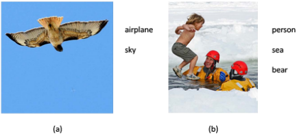

This paper is motivated to address both requirements for developing a robust multi-view tagging method. First, we want to make use of the unlabeled data through a semiparametric regularization. In particular, we consider the case where the unlabeled data are expected to determine the marginal distribution of the data if there is a small set of labeled data available along with a relatively large set of unlabeled data. Thus, we must consider the geometric structure of the marginal distribution of the whole data including the labeled data and the unlabeled data. Moreover, semi-parametric regularization are applied to explore the geometric structure of the whole data.
Second, we want to mitigate the influence of noisy tags by exploiting the whole information contained in the tag space. Figure 2 shows exemplar images with multiple tags. The images in the first row in Figure 2, which are all tagged as bird, always have the accompanied tags of sky, cloud, and tree, while the images in the second row in Figure 2, which are all tagged as fish, always have the accompanied tags of water, coral, and ocean. Obviously, these accompanied tags can be utilized as an additional feature to help better distinguish images tagged as bird from images tagged as fish. However, in the one-vs-all (OVA) mode, most of the Support Vector Machine (SVM)-based methods only utilize one tag of the data at a time, and ignore the other tags the data contain at the same time. For multi-view learning, since the multi-label space, which is the constitution of accompanied tags, can be considered as an additional shared feature between different views, we make use of it to build multi-label space consistency between samples from different views to mitigate the influence of the noise.
In this paper we investigate the multi-view tagging problem with a new perspective of considering semi-parametric regularization and multi-label space consistency simultaneously. In particular, we present Multi-view Semi-parametric Support Vector Machine with Multi-label Space Consistency (referred as MSMC), a discriminative method for multi-view tagging. The key idea lies in incorporating the geometric structure of the unlabeled data with the semi-parametric regularization and extending the similarity constraints between predictions on the samples from multiple views with the multi-label space consistency constraint.
While MSMC is a general method, we demonstrate through extensive evaluations in the application of multi-view image tagging using real data that the proposed method performs well in comparison with the peer methods in the literature as an effective and promising solution to the problem of semi-supervised multi-view learning with limited and noisy image tagging.
2 Related work
We begin by reviewing the literature on semi-supervised learning and multi-view learning, and then review the related work on the tagging methods. Finally, we introduce the literature in the field of noisy learning.
Most existing semi-supervised learning methods have been casted as a regularization problem in the literature. As a representative method, transductive SVM [Vapnik, 1998; Xu et al., 2007] is considered as combining fully supervised SVM with an additional regularization term on the unlabeled data. Semi-parametric regularization is also an attractive solution to semi-supervised problems [Smola et al., 1998; Ruppert et al., 2003; Guo et al., 2008; Bouboulis et al., 2010; Li et al., 2013].
Multi-view learning utilizes the consensus among learners trained on different views to improve the overall classification result [Xu et al., 2013]. It has been extensively used in the applications where data representations by multiple views exist [Sindhwani and Rosenberg, 2008; Rosenberg et al., 2009; Li et al., 2010; Liu et al., 2015]. Farquhar et al. [Farquhar et al., 2006] proposes SVM-2K by imposing a similarity constraint between two distinct SVMs each trained from one view of the data.
Tagging methods in the literature are mainly categorized into two types: generative methods and discriminative methods [Blei and Jordan, 2003; Zha et al., 2008; Zhang and Zhou,
2014]. Most generative methods introduce a set of latent variables to learn the joint distribution of the image features and semantic labels [Barnard et al., 2003]. Discriminative methods reduce the multi-label problem to a set of binary classification problems. The representative techniques for this category of approaches are extensions of SVM, which have demonstrated a strong discriminative power [Goh et al., 2001; Qi and Han, 2007; Yang et al., 2006].
Noisy tagging refers to scenarios of attribute noise and class noise [Zhu and Wu, 2004]. In this paper, we concentrate on the problem raised by class noise. There are a number of denoising methods for classification; they can be further classified into two categories: filtered preprocessing of the data and robust design of the algorithms. In the former category, filtered preprocessing is developed to remove the noise from the training set as much as possible [Van Hulse and Khoshgoftaar, 2006; Zhu et al., 2003]. For the latter category, robust algorithms are designed to reduce the impact of the noise in the classification [Lin and de Wang, 2004; Liu and Zheng, 2007; Tang et al., 2011; Qi et al., 2012]. Qi et al. [Qi et al., 2012] proposes a multi-view noisy tagging method, called MSS-2K, which exploits the information from a multi-label space. Further, they introduce an active learning scheme called MITL to improve the performance of MSS-2K. In addition, tag refinement is considered as the auxiliary work for image noisy tagging in the literature [Wang et al., 2007; Zhu et al., 2010; Liu et al., 2010].
3 Semi-parametric Regularization Learning Semi-parametric Regression
In statistics, semi-parametric regression refers to regression models that combine parametric and nonparametric models.
For example, suppose that we want to estimate an unknown function from a set of labeled data points (xi↪ yi), 1 i l by minimizing
where L(·) is a loss function.
Then for parametric regression models, ¯ f can be given as an explicit function which is dependent on a finite number of parameters (e.g., linear regression); for non-parametric regression models, ¯ f(x) cannot be estimated via an explicit function; for semi-parametric regressionmodels, ¯ f can be decomposed into two parts as ¯ f , f + h, where f is a nonparametric part which can be estimated from the data set, h 2 span¶ p♦Mp=1 , where ¶ p♦Mp=1 : X ! R is a family of parametric functions.
Minimizing the framework in Eq. (1) may lead to numerical instabilities and a bad generalization performance [Sch¨olkopf and Smola, 2001]. A possible solution is to add stabilization (regularization) term to the above minimization problem. This leads to a better conditioning of the problem. Thus, we consider the following minimization problem
where γ1 > 0 and γ2 > 0 are regularization parameters. When we equivalently think the feature space as a reproducing kernel Hilbert space, ⌦1[f] is the norm of the RKHS HK representation of the feature space kfk2K . ⌦2[h] is the norm of the parametric space khk2 , where k · k is the norm in , span¶ p♦Mp=1 . In this case, we equivalently minimize
where ¯ f , f +h with f 2 HK, and h 2 .
The following semi-parametric Representer Theorem states that the solution to the minimization problem in Eq. (3) exists in HK and , and gives the explicit form of a minimizer.
Theorem 1. (Semi-parametric Representer Theorem [Sch¨olkopf and Smola, 2001]): Denote by ⌦ : [0↪ 1) ⇥ [0↪ 1) ! R a strictly monotonically increasing function, by X a set, and by c : (X ⇥ R2 )l ! R [ ¶1♦ an arbitrary loss function. Let ¶ p♦Mp=1 : X !R be a set of M real valued functions with the property that the l ⇥M matrix ( p(xi))ip has rank M and span¶ p♦ , ⇢ H?K has the norm k · k . Then for any ¯ f , f + h with f 2 HK and h 2 , minimizing the regularized risk
with ↵i↪ βp 2 R.
Learning Parametric Functions
Let x1↪ ▷ ▷ ▷ ↪ xl+υ 2 Rd denote a set of inputs including l labeled data points and υ unlabeled data points. For semiparametric regression, we might hope that the geometric structure of the whole data distribution can be exploited for a better function learning. There are suitable choices for the parametric functions. Specifically, we adopt the same strategy as that in [Guo et al., 2008] to obtain the parametric functions by applying Kernel Principal Component Analysis (KPCA) algorithm [Sch¨olkopf et al., 1997] to the whole data set. KPCA finds the principal axes in the feature space which carry more variance than any other directions by diagonalizing the covariance matrix.
where φ is a mapping function in the RKHS.
To find the principal component, we solve the eigenvalue problem, ⌃W = ⇤W. Let ⇤ denote the M largest eigenvalues and W the corresponding eigenvector space. Given the data point x, the projection onto the principal axes is given by φ(x)T W. Therefore, we can set the parametric function for φ(x):
SinceW is a linear combination of the kernel functions in RKHS, the geometric structure of the marginal distribution of the data can be obtained by this learned parametric function. Further, the geometric structure of the data distribution is incorporated by a semi-parametric regularization. In this way, we obtain the minimizer of Eq. (3) as follows:
where K is the kernel in the original RKHS HK.
3.1 Semi-parametric SVM
Based on the above derivation, we extend the standard SVM to semi-parametric SVM by solving the following optimization problem:
where β = (β1↪ ▷ ▷ ▷ ↪ βM+1) and (xi) = (1↪ 1(xi)↪ ▷ ▷ ▷ ↪ M(xi)). In particular, the semi-parametric SVM reduces to the standard SVM when M = 0.
4 Multi-view Semi-parametric SVMwith Multi-label Space Consistency
4.1 Notations for Multi-label Space
In this paper we concentrate on the two-view case. It is easy to extend the proposed method to more than two views. Two views of the dataset I are denoted as V (a) and V (b) , respectively. Each instance Ii 2 I is labeled with various tags. The whole tag vocabulary for I forms the E-dimensional multilabel space T . When one tag Tr (1 r E) is chosen as the classification target, the other tags can form the additional feature space of tags, denoted as Lr. Obviously, the dimensionality of Lr is E - 1. Let an E-dimensional vector di = (di↪1↪ di↪2↪ ▷ ▷ ▷ ↪ di↪E)0 be the tag representation for Ii, where di↪r 2 ¶0↪ 1♦↪ 1 r E represents the occurrence of the rth tag Tr for Ii. For each Ii and each Tr, we denote yi↪r as the class label of Ii, where yi↪r = 2 · di↪r - 1. Ii = (x(a) i ↪ x(b) i ↪ di), where x(a) i and x(b) i are the feature descriptors of Ii.
4.2 Motivation of MSMC
In the two views learning, we assume that the labeled data are of the following formulation: Ii = ¶x(a) i ↪ x(b) i ↪ yi♦ni=1 , where x(a) i (x(b) i ) is a feature vector of Ii in view V (a) (V (b) ), and yi 2 ¶-1↪+1♦ is a class label of Ii. The classical SVM-2K imposes a similarity constraint between two distinct SVMs each trained from one view of the data. The constraint they introduce into the optimization is
where f (a)∩(b) (·) are the SVM decision functions belonging to each of the two views by superscripts a and b, respectively, ⌘i is a variable that improves the consensus between the two views.
A first approach to multi-view semi-parametric learning is to combine the above constraint with the semi-parametric SVM objective function for each view,
where ¯ f (a)∩(b) (·) are the semi-parametric SVM decision functions belonging to each of the two views by superscripts a and b, respectively.
However, this model suffers from the limitation that it cannot exploit the information contained in the tag space. Assume that we have three images, where the first has tags motor, people, and road, the second has tags people and road, and the third has tags people, TV, and office. When the tag people is chosen as the classification target, the second image is more similar to the first one than the third one because it shares road with the first image while the third image has no road. From this point of view, the traditional multi-view learning methods that ignore the tag information may not be appropriate.
Specifically, in the OVA mode, when one tag Tr is chosen as the classification target, the other tags can form the additional feature space of the tags Lr. We denote the feature vector of Ii in Lr as ti↪r, where ti↪r = (di↪1↪ ▷ ▷ ▷ ↪ di↪r-1↪ di↪r+1↪ ▷ ▷ ▷ ↪ di↪E)0 . The neighborhood of Ii in Lr ( including Ii itself) is denoted as Nr(Ii). The neighborhood information can then be added into the learning between the views by introducing the following consistency constraints:
where Ni , ¶j♣Ij 2 Nr(Ii)♦. We show that constraint (12) can be approximately obtained by constraint (11). For i 2 Nj , constraint (11) works. For i ◁2 Nj, we obtain the following constraint based on constraint (11):
From the above inference, constraint (12) coincides with constraint (11) approximately with a little larger constraint variable. Thus, we only select constraint (11) in order to reduce the computational complexity.
4.3 Formulation of MSMC
Combining the two-view constraint (11) with the semiparametric SVM and allowing different regularization constants, we obtain the following optimization for multi-view semi-parametric SVM with multi-label space consistency (MSMC):
where Sim(ti↪r↪ tj↪r) represents the Jaccard similarity coefficient between Ii and Ij in Lr.
Based on the above analyses, the algorithm of MSMC is outlined in Algorithm 1.
Algorithm 1: MSMC Algorithm
Input : Datasets X(a) L , X(b) L , X(a) U , and X(b) U ; XL is the labeled set; XU is the unlabeled set.
Output: Estimated function ¯ f (a) and ¯ f (b) .
- 1 Choose the kernel K and do KPCA on the whole data set; get (x) with Eq.(6);
- 2 Solve the convex optimization problem in Eq.(14) with quadratic programming[Gill and Wong, 2015];
- 3 Output ¯ f (a) (x) and ¯ f (b) (x);
Computation Complexity Analysis. From the algorithm flowchart we see that the main computational cost of MSMC lies in two parts: (1) to perform KPCA on the whole dataset; (2) to solve the optimization problem (14). Conventionally, the first part costs O(n3 ), where n = l+υ is the total number of data points, and the second part costs O(P 3 ), where P is the size of the support vectors. P ⇡ uQ, where u is the size of the neighborhood in the paper and Q is the size of the support vectors of the traditional SVM-2K. Practically, u = 4 is sufficient to secure a good performance.
5 Experiments
5.1 Data and Parameter Setting
While MSMC is a general method for multi-view learning with limited and noisy tagging, we report the extensive evaluations in the specific application of multi-view noisy image tagging with limited labeled training samples. We compare our method with SVM, Semi-parametric SVM (Sp-SVM) [Guo et al., 2008], fuzzy SVM [Lin and de Wang, 2004], SVM-2K [Farquhar et al., 2006], Co-training, and MSS-2K
[Qi et al., 2012] using the noisily tagged training images combined with the plentiful untagged images to evaluate the performances of these methods.
The NUS-WIDE [Chua et al., 2009] image dataset is used in the experiments. It includes 269↪ 648 web images and 81 concepts which we treat as the ground truth tags. We choose the top 75 concepts whose numbers of positive examples are larger than 200 from the dataset to form the multi-label space T . Hence, the dimensionality of the additional feature space of tags (Lr) for each Tr is 74. For each concept, we randomly choose 260 positive examples and 260 negative examples as the training data. In the testing set, the numbers of the positive and negative examples are both 50. 10% examples are randomly selected from the training data to form the perfectly tagged training set, and the left 90% examples from the training data are used as the untagged training set. In the experiments, s% noise is added into both the positive and negative examples of the perfectly tagged training set to form the noisily tagged training set. We denote the 500-D bag of words feature based on SIFT descriptions as Va, and denote the 1000-D bag of text words feature which describes the text information correlated to the images provided by the dataset as Vb.
The size u of the neighborhood Nr(Ii) for each Ii is defined as the count of the nearest neighbors of Ii in Lr. Further, the nearest neighbors of Ii is computed with the Jaccard similarity coefficient between Ii and other samples in Lr. We define R as the ratio between the weight of the loss function for instances and in the weight of the loss function for their nearest neighbors in the optimization. For MSMC, R = C (ab) ◁C (a)∩(b) , where C (a) = C (b) . In the experiments, we choose the top M largest eigenvalues and the corresponding eigenvectors from the results of KPCA to learn the parametric function for the training data. M = 0 means that we learn no parametric function for the training data.
5.2 EvaluationMetric
For each tag Tr, let CTr be the number of correctly predicted examples, GTr be the number of the examples which actually have the tag as the ground truth, and PTr be the number of all the predicted examples with the tag. Then the precision Prer, recall Recr, and F1 measure are defined as
We evaluate the performances of the methods using the standard performance measures of Macro-F1 (F1a ) and MicroF1 (F1i ). Macro-F1 averages the F1 measures on the predictions of different tags; Micro-F1 computes the F1 measure on the predictions of different labels as a whole.
5.3 Performance Comparisons
In Table 1, we summarize the F1 measure of the testing set when M = 3, u = 4, R = 0▷5, and s is selected as 30, 25, 20,
15, 10, and 5 in the two views combined, for SVM, Sp-SVM, fuzzy SVM, Co-training, SVM-2K, MSS-2K, and MSMC, respectively. For each method, we obtain the combined prediction with the simple average strategy on the two views' prediction. On the task of multi-view learning with limited and noisy image tagging, compared with MSMC, SVM with the noisily tagged training set considers the training set as the perfectly tagged set and mistakenly takes the incorrect tags as the perfect tags. Although Sp-SVM exploits the geometric structure of the unlabeled data, it considers the training set as the perfectly tagged set and cannot take advantage of the information from the multi-label space. Fuzzy SVM considers the training set as noisily tagged dataset, but it cannot take advantage of the information contained in multi-label space and untagged data set. Although Co-training takes advantage of the information from the untagged data, it considers the training set as the perfectly tagged set and fails to make use of the information from the multi-label space. Similarly, SVM2K also considers the training set as the perfectly tagged set, and fails to make use of the information from the multi-label space. Further, though MSS-2K utilizes the information contained in the multi-label space by imposing more constraints between multiple view learners, it fails to take advantage of the information contained in the untagged data to make it adaptive to the environment with limited and noisy training data. Consequently, from Table 1, we see that MSMC performs better than SVM, fuzzy SVM, Co-training, SVM-2K and MSS-2K on the task of multi-view learning with limited and noisy image annotation in all the cases as the F1 measures achieved by MSMC are much higher than those achieved by the competing models in all cases.
Specially, when s is selected as 30, 25, 20, MSMC performs better than the competing models significantly. It demonstrates the robustness of MSMC when the training set is seriously noisy.
5.4 Sensitivity Study
We conduct a sensitivity study on the proposed MSMC algorithm. In particular, we study how the semi-parametric parameter, the neighborhood size, and the regularization parameter affect the performance of MSMC, respectively.
We describe the F 1 measure for the testing set as a function of M when u = 4, R = 0▷5, and s = 20 using the combination of feature Va and feature Vb for MSMC in Figure 3(a). From Figure 3(a), we observe that the F1 measures for the testing set increase when M increases, which shows that the semi-parametric regularization is helpful to further improve the performance of the classification by better exploiting the geometric structure of the marginal distribution of the data. The curves for the F1 measures of MSMC in Figure 3(a) exhibit the major effect from M = 0 to M = 1, and then are stable when M continues to increase. This is because M=1 corresponds to the most discriminative component in the data distribution. It is also a well-known fact that most of the existing semi-parametric learning methods are implemented with M = 1 [Guo et al., 2008].
Figure 3(b) shows the F1 measures for the testing set as a function of u when M = 3, R = 0▷5, and s = 20 using the combination of feature Va and feature Vb for MSMC. From MSMC 0▷7368∩0▷7600 0▷7628∩0▷7675 0▷7748∩0▷7840 0▷7992∩0▷8055 0▷8285∩0▷8305 0▷8392∩0▷8384
Table 1: The F1 measures for the testing set.
| F1a ∩F1i using the combination of feature Va and feature Vb | ||||||
|---|---|---|---|---|---|---|
| s = 30 | s = 25 | s = 20 | s = 15 | s = 10 | s = 5 | |
| SVM | 0▷6302∩0▷6536 | 0▷6852∩0▷7031 | 0▷7279∩0▷7398 | 0▷7799∩0▷7858 | 0▷8091∩0▷8114 | 0▷8250∩0▷8261 |
| Sp-SVM | 0▷6436∩0▷6664 | 0▷6996∩0▷7163 | 0▷7381∩0▷7487 | 0▷7895∩0▷7953 | 0▷8151∩0▷8172 | 0▷8316∩0▷8327 |
| Fuzzy SVM | 0▷6209∩0▷6426 | 0▷6901∩0▷7073 | 0▷7219∩0▷7325 | 0▷7725∩0▷7808 | 0▷8029∩0▷8059 | 0▷8220∩0▷8238 |
| SVM-2K | 0▷6295∩0▷6451 | 0▷6735∩0▷6891 | 0▷7250∩0▷7332 | 0▷7714∩0▷7762 | 0▷8047∩0▷8054 | 0▷8179∩0▷8190 |
| Co-training | 0▷6693∩0▷6883 | 0▷7134∩0▷7267 | 0▷7489∩0▷7596 | 0▷7944∩0▷8003 | 0▷8161∩0▷8182 | 0▷8307∩0▷8326 |
| MSS-2K | 0▷6396∩0▷6600 | 0▷6972∩0▷7154 | 0▷7449∩0▷7539 | 0▷7869∩0▷7925 | 0▷8148∩0▷8165 | 0▷8278∩0▷8282 |
| MSMC | ||||||
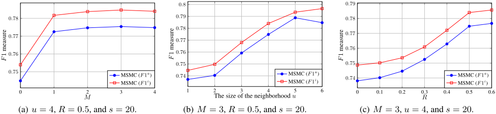
Figure 3(b), we observe that the F1 measures for the testing set increase when the size of the neighborhood for each Ni increases, which shows that it is helpful to use the nearest neighbors of each Ii in Lr to further improve the performance of the classification.
We describe the F 1 measure for the testing set as a function of R when M = 3, u = 4, and s = 20 using the combination of feature Va and feature Vb for MSMC in Figure 3(c). As we defined before, R = C (ab) ◁C (a)∩(b) represents the ratio between the weight of the loss function for their nearest neighbors and the weight of the loss function for instances in the corresponding views. We observe from Figure 3(c) that when R increases, the curves for the F1 measures of MSMC ascend, which also shows that it is helpful to use the nearest neighbors of each Ii in Lr to reduce the influence of the noise in the classification.
6 Conclusion
In this paper, we have studied the challenging problem of multi-view learning with limited and noisy tagging and have developed a powerful discriminative model, called MSMC, that exploits both labeled and unlabeled data through a semiparametric regularization and takes advantage of the multilabel constraints into the optimization. While MSMC is a general method for multi-view learning with limited and noisy tagging, we have reported the extensive evaluations in the specific application of multi-view noisy image tagging with limited labeled training samples on a benchmark dataset. Extensive evaluations in comparison with the state-of-the-art literature demonstrate that MSMC outstands with a superior performance.
7 Acknowledgments
This work was supported in part by the National Basic Research Program of China under Grant 2012CB316400, Zhejiang Provincial Engineering Center on Media Data Cloud Processing and Analysis, and equipment donation by Nvidia. Z. Xu was also supported by NSF China (No. 61572111, 61433014, 61440036), a 985 Project of UESTC (No.A1098531023601041) and Basic Research Projects of China Central Universities ( No. ZYGX2014J058, A03012023601042).
@inproceedings{ijcai2016p246,
  title     = {Multi-View Learning with Limited and Noisy Tagging},
  author    = {Li, Yingming and Yang, Ming and Xu, Zenglin and Zhang, Zhongfei},
  booktitle = {Proceedings of the Twenty-Fifth International Joint Conference on
               Artificial Intelligence, {IJCAI-16}},
  publisher = {AAAI Press / International Joint Conferences on Artificial Intelligence},
  editor    = {Subbarao Kambhampati},
  pages     = {1718--1723},
  year      = {2016},
  month     = {7},
  url       = {https://ijcai.org/proceedings/2016/246},
}
TY - CPAPER TI - Multi-View Learning with Limited and Noisy Tagging AU - Li, Yingming AU - Yang, Ming AU - Xu, Zenglin AU - Zhang, Zhongfei T2 - Proceedings of the Twenty-Fifth International Joint Conference on Artificial Intelligence, IJCAI-16 PB - AAAI Press / International Joint Conferences on Artificial Intelligence PY - 2016 SP - 1718 EP - 1723 UR - https://ijcai.org/proceedings/2016/246 ER -Copied
Machine-readable versions of this paper, for tools and AI agents:





