
Fast Laplace Approximation for Sparse Bayesian Spike and Slab Models
Proceedings of the Twenty-Fifth International Joint Conference on Artificial Intelligence. Pages 1867-1972.
Abstract
We consider the application of Bayesian spike-and-slab models in high-dimensional feature selection problems. To do so, we propose a simple yet effective fast approximate Bayesian inference algorithm based on Laplace's method. We exploit two efficient optimization methods, GIST and L-BFGS, to obtain the mode of the posterior distribution. Then we propose an ensemble Nystrom based approach to calculate the diagonal of the inverse Hessian over the mode to obtain the approximate posterior marginals in O(knp) time, k ≪ p. Furthermore, we provide the theoretical analysis about the estimation consistency and approximation error bounds. With the posterior marginals of the model weights, we use quadrature integration to estimate the marginal posteriors of selection probabilities and indicator variables for all features, which quantify the selection uncertainty. Our method not only maintains the benefits of the Bayesian treatment (e.g., uncertainty quantification) but also possesses the computational efficiency, and oracle properties of the frequentist methods. Simulation shows that our method estimates better or comparable selection probabilities and indicator variables than alternative approximate inference methods such as VB and EP, but with less running time. Extensive experiments on large real datasets demonstrate that our method often improves prediction accuracy over Bayesian automatic relevance determination, EP, and frequentist L1 type methods.
- [Ahmed and Xing, 2009] Amr Ahmed and Eric P Xing. Re- covering time-varying networks of dependencies in so- cial and biological studies. Proceedings of the National Academy of Sciences, 106(29):11878-11883, 2009.
- [Bezdek and Hathaway, 2003] James C Bezdek and Richard J Hathaway. Convergence of alternating optimization. Neu- ral, Parallel & Scientific Computations, 11(4):351-368, 2003.
- [Candès, 2006] Emmanuel J Candès. Compressive sampling. In Proceedings oh the International Congress of Mathe- maticians: invited lectures, pages 1433-1452, 2006.
- [Carbonetto et al., 2012] Peter Carbonetto, Matthew Stephens, et al. Scalable variational inference for bayesian variable selection in regression, and its accuracy in genetic association studies. Bayesian Analysis, 7(1):73-108, 2012.
- [Gong et al., 2013] Pinghua Gong, Changshui Zhang, Zhaosong Lu, Jianhua Huang, and Jieping Ye. A general iterative shrinkage and thresholding algorithm for non- convex regularized optimization problems. In The 30th International Conference on Machine Learning, pages 37-45, 2013.
- [Hernández-Lobato et al., 2010a] Daniel Hernández-Lobato, José Miguel Hernández-Lobato, Thibault Helleputte, and Pierre Dupont. Expectation propagation for bayesian multi- task feature selection. In Machine Learning and Knowledge Discovery in Databases, pages 522-537. Springer, 2010.
- [Hernández-Lobato et al., 2010b] Daniel Hernández-Lobato, José Miguel Hernández-Lobato, and Alberto Suárez. Ex- pectation propagation for microarray data classification. Pattern recognition letters, 31(12):1618-1626, 2010.
- [Hernández-Lobato, 2010] José Miguel Hernández-Lobato. Balancing flexibility and robustness in machine learning semi-parametric methods and sparse linear models. PhD thesis, Ph. D. Thesis, Universidad Autó De Madrid, 2010.
- [Hoerl and Kennard, 1970] Arthur E Hoerl and Robert W Kennard. Ridge regression: Biased estimation for nonorthogonal problems. Technometrics, 12(1):55-67, 1970.
- [Ishwaran and Rao, 2005] Hemant Ishwaran and J Sunil Rao. Spike and slab variable selection: frequentist and bayesian strategies. Annals of Statistics, pages 730-773, 2005.
- [Kogan et al., 2009] Shimon Kogan, Dimitry Levin, Bryan R Routledge, Jacob S Sagi, and Noah A Smith. Predicting risk from financial reports with regression. In Proceedings of Human Language Technologies: The 2009 Annual Con- ference of the North American Chapter of the Association for Computational Linguistics, pages 272-280. Association for Computational Linguistics, 2009.
- [Kumar et al., 2009] Sanjiv Kumar, Mehryar Mohri, and Ameet Talwalkar. Ensemble nystrom method. In Advances in Neural Information Processing Systems, pages 1060- 1068, 2009.
- [Minka, 2000] Thomas P Minka. Deriving quadrature rules from Gaussian processes. Technical report, Statistics De- partment, Carnegie Mellon University, 2000.
- [Mitchell and Beauchamp, 1988] Toby J Mitchell and John J Beauchamp. Bayesian variable selection in linear regres- sion. Journal of the American Statistical Association, 83(404):1023-1032, 1988.
- [Nocedal, 1980] Jorge Nocedal. Updating quasi-newton ma- trices with limited storage. Mathematics of computation, 35(151):773-782, 1980.
- [Qi et al., 2005] Y. Qi, T. S. Jaakkola, and D.K. Gifford. Ap- proximate expectation propagation for bayesian inference on large-scale problems. Technical report, MIT Com- puter Science and Artificial Intelligence Laboratory, Octo- ber 2005.
- [Rosenwald et al., 2002] Andreas Rosenwald, George Wright, Wing C Chan, Joseph M Connors, Elias Campo, Richard I Fisher, Randy D Gascoyne, H Konrad Muller- Hermelink, Erlend B Smeland, Jena M Giltnane, et al. The use of molecular profiling to predict survival after chemotherapy for diffuse large-b-cell lymphoma. New England Journal of Medicine, 346(25):1937-1947, 2002.
- [Rue et al., 2009] Hravard Rue, Sara Martino, and Nicolas Chopin. Approximate bayesian inference for latent gaussian models by using integrated nested laplace approximations. Journal of the royal statistical society: Series b (statistical methodology), 71(2):319-392, 2009.
- [Scheetz et al., 2006] Todd E Scheetz, Kwang-Youn A Kim, Ruth E Swiderski, Alisdair R Philp, Terry A Braun, Kevin L Knudtson, Anne M Dorrance, Gerald F DiBona, Jian Huang, Thomas L Casavant, et al. Regulation of gene ex- pression in the mammalian eye and its relevance to eye dis- ease. Proceedings of the National Academy of Sciences, 103(39):14429-14434, 2006.
- [Tibshirani, 1996] Robert Tibshirani. Regression shrinkage and selection via the lasso. Journal of the Royal Statistical Society. Series B (Methodological), pages 267-288, 1996.
- [Titsias and Lázaro-Gredilla, 2011] Michalis K Titsias and Miguel Lázaro-Gredilla. Spike and slab variational infer- ence for multi-task and multiple kernel learning. In NIPS, volume 24, pages 2339-2347, 2011.
- [Woodbury, 1950] Max A Woodbury. Inverting modified ma- trices. Memorandum report, 42:106, 1950.
- [Yen, 2011] Tso-Jung Yen. A majorization-minimization ap- proach to variable selection using spike and slab priors. The Annals of Statistics, 39(3):1748-1775, 2011.
- [Zhe et al., 2013] Shandian Zhe, Syed AZ Naqvi, Yifan Yang, and Yuan Qi. Joint network and node selection for pathway- based genomic data analysis. Bioinformatics, 2013.
- [Zou and Hastie, 2005] Hui Zou and Trevor Hastie. Regular- ization and variable selection via the elastic net. Journal of the Royal Statistical Society: Series B (Statistical Method- ology), 67(2):301-320, 2005.
- [Zou and Zhang, 2009] Hui Zou and Hao Helen Zhang. On the adaptive elastic-net with a diverging number of parame- ters. Annals of statistics, 37(4):1733, 2009.
References were extracted automatically from the PDF and may contain errors.
Full text extracted automatically from the PDF; figures, tables and equations may differ. The PDF is the version of record.
1 Introduction
As an intersection of machine learning, statistics, and signal processing, sparse modeling has numerous applications. For developing various sparse models, L1 regularization has played a central role. L1-type methods not only enjoy provable properties relating to the estimation optimality and oracle properties [Zou and Hastie, 2005; Tibshirani, 1996], but also have the convenience of using welldeveloped computational tools from convex optimization to obtain sparse solutions. As a result, they have been widely used in many applications including feature selection, compress sensing[Cand`es, 2006], multi task learning [Titsias and L´azaro-Gredilla, 2011], and time-varying network reconstruction [Ahmed and Xing, 2009].
Recently there has been a shift from convex to nonconvex regularization approaches in the machine learning community. Specifically, within the Bayesian context, the spikeand-slab prior has been the focus of attention due to its selective shrinkage property. In this paper, we examine the performance of the Bayesian spike-and-slab models for very high dimensional problems in the supervised learning setting. For very high dimensional problems, existing Monte Carlo methods [Mitchell and Beauchamp, 1988] converge slowly with tens of thousands of features in data; and the variational Bayes (VB) and expectation propagation (EP) approaches [Hern´andez-Lobato et al., 2010a; Hern´andez-Lobato, 2010; Hern´andez-Lobato et al., 2010b] either need a fully factorized approximation to obtain a linear cost, but at the price of a reduced approximation quality, or have a quadratic cost, making them impractical for large data. By contrast, the frequentist L1-type methods have fast solvers developed over years, making them a practical tool. To address the computational issue associated with the spike-and-slab model, we develop the Fast Laplace Approximation for Spike-and-slab (FLAS) algorithm. Our approach not only maintains the benefits of the Bayesian treatment (e.g., uncertainty quantification) but also possesses the computational efficiency, and oracle properties of the frequentist methods.
Specifically, in Section 3, we apply the Laplace approximation to the marginal posterior distribution of each weight parameter. For the Laplace approximation we need to obtain the mode of the posterior distribution. To this end, we exploit two efficient optimization methods, the popular limitedmemory BFGS (L-BFGS) [Nocedal, 1980] and the recently developed GIST method [Gong et al., 2013]. Specifically, we use L-BFGS to obtain the MAP estimation for the marginalized model, and we use an alternating optimization strategy based on GIST [Gong et al., 2013] for the joint model, with convergence guarantees for both regression and classification, and possessing oracle properties for the regression case. Then we propose an ensemble Nystr¨om based approach to calculate the diagonal of the inverse Hessian over the mode to obtain the approximate posterior marginals in O(knp) time, where n and p are the numbers of samples and features respectively, and k ⌧ p. The theoretical analysis of the ensemble method is also provided. With the posterior marginals of model weights, we use quadrature integration to estimate the marginal posteriors of selection probabilities and indicator variables for all features, which quantify the selection uncertainty. While a factorized joint posterior assumption is usually not true, VB and EP often adopt it for computational efficiency. By contrast, our method is free of this assumption but still enjoys a cost linear in p. Detailed discussion on the related work is given in Section 4.
On simulated data, our methods perform feature selection better than or comparable to the alternative approximate methods, with less running time, and provide higher prediction accuracy than various sparse methods (Section 5). On large real benchmark datasets, our methods often achieve improved prediction accuracy with a comparable speed.
2 Spike-and-SlabModels
We first present sparse linear models with spike-and-slab priors. Suppose we have n independent and identically distributed samples D = ¶(x1↪ t1)↪ ▷ ▷ ▷ ↪ (xn↪ tn)♦, where xi is the p dimensional feature vector of the i-th sample, and ti is its response. We aim at predicting the response vector t = [t1↪ ▷ ▷ ▷ ↪ tn]> based on the feature set X = [x1↪ ▷ ▷ ▷ ↪ xn]> and selecting a small number of features relevant to the prediction. For real-world applications, we often have n ⌧ p.
A set of latent binary variables ¶zj♦ are introduced to indicate the feature selection: zj = 1 means the j-th feature is selected; otherwise, it is not. Then a spike-and-slab prior [Ishwaran and Rao, 2005] over w is assigned:
For regression, the Gaussian data likelihood is used: p(t♣X↪ w↪ ⌧ ) = Qni=1 N(ti♣x>i w↪ ⌧ -1 ) where w are regression weights, and ⌧ is the precision parameter; for classification, the logistic likelihood is used: p(t♣X↪w) = Qni=1 σ(x>i w)ti [1 - σ(x>i w)]1-ti where ti 2 ¶0↪ 1♦, w are classifier weights, and σ(a) = 1◁(1 + exp(-a)).
where r0 and r1 are the variances of the two Gaussian components and sj 2 [0↪ 1] represents the selection probability for the j-feature. We set r1 ≫ r0 so that if the j-th feature is selected, the prior over wj has a large variance r1 (as a regular L2 penalty in the frequentist framework) and, if not, the zeromean prior has a very small variance r0, leading to aggressive shrinkage of the irrelevant feature. We further assign a Beta prior over sj: p(sj) = Beta(a0↪ b0). In the experiments, we set a0 = b0 = 1 such that this prior is an uninformative uniform prior.
3 Algorithm
Given high dimensional data, current inference methods such as Gibbs sampling or VB can suffer from high computational cost. To overcome the computational bottleneck, we use Laplace's method to approximate the posteriors of each ¶wj♦ and apply the quadrature integration [Minka, 2000] to estimate the selection probability sj and indicator variable zj .
3.1 Laplace approximation
To obtain the Laplace approximation, we need to compute the mode and the second-order derivative of the log posterior distribution at the mode. We describe two approaches for computing MAP estimation: marginalized MAP estimation ,and joint MAP estimation. Details of the two approaches are described below.
L-BFGS optimization of the marginalized model
For the first approach, denoted by FLAS, we marginalize out both z and s. The negative log probability of the marginalized model is then given by
where L(w) is the negative log likelihood for regression or classification. To minimize the negative log probability, we use the L-BFGS method [Nocedal, 1980] because of its low computational and memory cost, and due to the nonconvexity of the spike-and-slab model. As a quasi-Newton method, the L-BFGS method uses last M function/gradient pairs to approximate the inverse Hessian matrix of the parameters w. Because M is set to be much smaller than p, often as small as 3-10, the computational cost per iteration is linear in p.
To use L-BFGS, we need to compute the gradient over w:
where g(wj) = q r1 r0 exp( 12 ( 1 r1 - 1 r0 )w2 j ), and dL(w) dw = ⌧X>(Xw - t), for regression and dL(w) dw = PNn=1 ( tn 1+exp(x>n w) - 1-tn 1+exp(-x>n w) )xn, for classification.
Using the gradient in the L-BFGS method, we can compute the mode of wj efficiently. Then we can approximate the posteriors of sj and zj as explained in Section 3.3.
Optimization of the joint model
For the second approach, denoted by FLAS*, we only marginalize out z and jointly optimize over the weights w and the selection probability s. From a Bayesian perspective, we prefer the first approach because by marginalizing out s, it essentially takes all possible values of s into account. But the second approach can provide a more pronounced selective shrinkage effect than the first approach. We use an alternating optimization (AO) approach for both regression and classification, and employ GIST [Gong et al., 2013] for finding the minimizer of w during the AO iterations.
In the joint optimization, we minimize the negative log joint probability:
where R(w↪ s) = Ppj=1 Rj(wj↪ sj) and Rj(wj↪ sj) = log (sjN (wj ♣0↪ r1) + (1 - sj )N (wj ♣0↪ r0)).
We perform alternating optimization by keeping one variable fixed, and optimize over the other. We start the optimization procedure by randomly initializing w. Given w as fixed, F(w↪ s) is a monotone function of each sj, hence it attains a minimum at sj = 1 if ♣wj♣ ≥ a, and sj = 0 otherwise, a = r⇣ 2r0r1 r1-r0 ⌘ log q r1 r0 . Given s, the optimization of w has a closed form solution for regression that is a special case of generalized ridge regression [Hoerl and Kennard, 1970]:
where d is such that dj = ( 1 r1 )sj ( 1 r0 )1-sj .
The update of w has a time complexity of O(p3 ). This is prohibitively expensive at higher dimensions. Therefore, we employ GIST to minimize w. Since the problem is strictly convex, GIST is guaranteed to converge to the unique minimum (closed form solution), but with cost per iteration O(np)[Gong et al., 2013]. In case of classification, we do not have have a closed form update for w, but with the logistic loss function the optimization problem is still strictly convex, hence GIST again converges to the unique minimum. Our AO scheme also satisfies the Existence and Uniqueness (EU) assumption, and hence converges to a joint local minimum [Bezdek and Hathaway, 2003].
Estimation, Selection and Sign consistency for regression
Using the approach given in [Yen, 2011] and [Zou and Zhang, 2009], we will prove asymptotic consistency properties for the AO estimator. Let us assume that w⇤ is the true coefficient vector of the regression model. Define S⇤ = ¶j : w⇤ j 6= 0♦, and Sopt = ¶j : woptj 6= 0♦. Let S denote the space in which S⇤ lies. Selection consistency implies that S⇤ = Sopt, and sign consistency requires sign(w⇤ ) = sign(wopt), where sign(a) = 1↪ 0↪-1 for a > 0↪ a = 0↪ a < 0 respectively, sign operator is applied component wise. We will use the following assumptions for our analysis:
Assumption 1 [Yen, 2011]. Let CSS = n-1 (X>S XS) for any S 2 S. Let λi be the ith eigenvalue of CSS, then the following condition holds:
Assumption 2. For parameters r1, r0 and ⌧, assume that they are fixed, and 0 < r1↪ r0↪ ⌧ < 1;
Assumption 4. Let x1↪ x2↪ ▷▷▷↪ xn be a sample from p dimensional Gaussian distribution N(0↪ Ip) with mean 0 and unit covariance matrix. Then, for sufficiently large n with p fixed, X>X ! nIp. Let ⇣ = X>✏ then there exist a finite positive constant ⇣0 such that ♣⇣i♣ < ⇣0 for all i = 1↪ ▷▷▷↪ p.
Assumption 3 [Yen, 2011]. Assume a finite constant c3 > 0 such that (w⇤ j )2 < c3 for all j = 1↪ ↪ · · · p.
Assumption 5. Assume that their exist a positive finite constant M such that ♣w⇤ i ♣ ≥ M, i 2 S⇤ . Also assume a small positive constant δ such that 0 < δ < M
Assumption 1 enforces positive definiteness of the sample covariance matrix. This assumption is reasonable for large sample sizes as the sample covariance matrix is of full rank. Assumption 2 simply indicates that we know the true value of the hyper parameters. However, our results are also valid for bounded support. Therefore, assuming the parameters as fixed and known is not necessary. Assumption 3 is needed to make sure that the true weight vector does not grow without bound. This is required because in theorem 1 the true weight vector changes with sample size. Assumption 4 can find its applications in situations where the user has control over the design of matrix X, for example compressed sensing. Assumption 5 enforces absolute shrinkage, and hence selection and sign consistency.
Theorem 1. Given that 1, 2, and 3 are satisfied and p / n↵ with ↵ > 0, then P(♣♣wopt - w⇤ ♣♣2 > ⇠n) c0 exp¶- log(n1-↵⇠n)♦ for some positive finite constants c0 and ⇠n. Assume that ⇠n / n-↵⇤ for some ↵⇤ > 0. Then if 0 < ↵⇤ < ↵ < 1◁2, P(♣♣wopt - w⇤ ♣♣2 > ⇠n) ! 0 as n !1, and hence wopt has estimation consistency.
Theorem 2. Under assumptions 2, 4, and 5 wopt ! w⇤ as n ! 1 with p fixed. Let wcopt = e ◦ wopt, where ei = 1 if ♣wopti♣ ≥ M - δ, and 0 otherwise. Then, wcopt will be sign and selection consistent as n ! 1 with p fixed. (All proofs are omitted due to space limitations)
3.2 Marginal Posterior of Weights
Standard Laplace approximation requires to invert the Hessian matrix of the negative log probability at the mode, via which we can obtain a joint approximate posterior. For prediction and feature selection, however, we only need marginal posterior of each weight wj , which only requires the diagonal entry of the inverse Hessian. Nevertheless, we still have to invert the Hessian matrix, which has time complexity of O(p3 ) and is unacceptable for large problems. To resolve this issue, we resort to Nystr¨om method. Specifically, let us denote the mode of the model weights by ˜w and consider the Hessian matrix in regression case first,
proach is used to approximate X>X: A subset of columns of X are sampled to form a low-rank n ⇥ k matrix Xk = [fi1 ↪ ▷ ▷ ▷ ↪ fik ], where fit is the it-th column of X; and X>X ⇡ X>Xk(X>k Xk) X>k X where (·) is the generalized inverse operation. The inverse of Hessian is then approximated by
Applying Woodbury matrix identity [Woodbury, 1950], we can readily reduce the complexity to O(nkp):
Since we can choose k ⌧ p, the inversion cost will still be linear in p. We can then read off the diagonal of ˜H-1 to calculate the marginal posterior approximation of each wj: a Gaussian with mean mj being the posterior mode ˜wj and variance σ2 j equal to the j-th entry of the diagonal of ˜H-1 .
For classification, the Hessian matrix has a slight different form: H = X>diag(b)X + diag(v), where bi = σ(x>i ˜w)(1-σ(x>i ˜w)). We can first multiply diag(pb) into X, i.e., ˜X=Xdiag(pb) and obtain H= ˜X> ˜X+diag(v). Then we follow the same way in regression case to calculate the Laplace approximation for each wj .
Using Nystr¨om approach to estimate the diagonal of inverse Hession will inevitably bring some approximation error. To improve accuracy, a simple ensemble approach is proposed. Specifically, we first sample d disjoint sets of columns of X, each set is of the same size k. For each set r, we can calculate an approximate inverse Hessian ˜H-1 r . The estimation of the j-th diagonal entry of inverse Hession is then obtained by
Using Taylor expansion and error bounds of Nystr¨om approximations[Kumar et al., 2009], we can prove that the proposed ensemble approach can have a smaller estimation error. This is expressed in the following theorems.
Theorem 3. Define ⌦ = ¶A 2 Rp⇥p ♣A ≻ 0↪ λmin(A) ≥ c↪ λmax(A) < 1♦. Assume Hessian H and rank-q Nystrom approximation of H based on k samples, ˜H, both belong to ⌦. Consider a function f(A) = e>j A-1ej↪A 2 ⌦. Then, krf(A)kF L, (1-⌘)H+⌘ ˜H 2 ⌦ 8 ⌘ 2 [0↪ 1], and with high probability,
where c is a small positive constant, and L = p◁c2 . ej is a standard basis vector with 1 in j-th coordinate and 0's elsewhere, and D0 is the Nystr¨om error bound based on Frobenius norm [Kumar et al., 2009].
Theorem 4. Define set S to be a collection of dk columns of Hessian H sampled uniformly at random without replacement, and partitioned into d subsets of size k, S1↪ · · · ↪ Sd. Assume Hessian H and d rank-q Nystrom approximations of H, ¶ ˜H1↪ ▷ ▷ ▷ ↪ ˜Hd♦ where ˜Hr denotes the rank-q Nystrom approximation of Hessian H based on the subset Sr, all belong to ⌦, then with high probability,
where D1 is the error bound for ensemble Nystr¨om based on Frobenius norm [Kumar et al., 2009]. Because D1 < D0 (see [Kumar et al., 2009]), the ensemble approach for the diagonal entry estimation of H-1 has a smaller error bound.
Proposition 1. Assume that λmax(X>X) < 1, and 8j c vj < 1. Then both Hessian H and any approximate Hessian ˜H based on Nystr ¨om method belong to ⌦, and hence satisfy theorems 3 and 4. (All proofs are omitted due to space limitations)
3.3 Posteriors moments of sj and zj
Given the approximate marginal posterior of wj, we can estimate marginal posterior moments of sj-the probability of selecting the j-th feature. Specifically, we first invert the conditional relationship between sj and wj based on Bayes rule,
Then the marginal posterior of sj can be computed by
where N (wj ♣mj ↪ σ2 j ) is the estimated posterior marginal of wj. Then, the posterior mean and variance of sj are calculated by
where Ng(wj) (for g = 0↪ 1) and q(wj) are the shorthand for N (wj ♣0↪ rg ) and N (wj ♣mj ↪ σ2 j ) respectively.
A similar procedure can be used to calculate the posterior moments of zj-the selection indicator of j-th feature; the poster mean and variance of zj are given by
We apply Gauss-Hermite quadrature method [Minka, 2000] to calculate the above one dimensional integrals with high accuracy. (e.g., the numerical difference from the true integration is often on the order of 10-4 ). The over all cost for computing the posterior mean and variance of w, s, and z is O(dknp), d↪ k ⌧ p. The linear cost makes our algorithm scalable for high dimensional data.
4 RelatedWork
A very closely related approach to our method proposes a MAP estimation of spike and slab models with delta spikes [Yen, 2011]. The method approximates the delta spike by a continuous bound via an elegant majorization and minimization (MM) algorithm. Consistency results for the MAP estimate are also provided. We, on the other hand, assume continuous spikes to make use of efficient continuous optimization strategies. Secondly, while the MM algorithm only focuses on the MAP estimate, we provide a full Bayesian inference strategy, and also show oracle properties for our MAP estimate. Another related method is the integrated nested Laplace approximation (INLA) [Rue et al., 2009]. INLA is designed for the latent Gaussian models and is shown to be very efficient and accurate. However, Spike-and-slab priors are mixture priors and do not belong to the latent Gaussian family. Simply applying INLA to the spike-and-slab models will be computationally expensive (O(p3 )) due to the dense precision matrix and high dimensional feature space.
EP and VB approximations have also been developed to conduct Bayesian inference on the spike-and-slab model. In the context of multi-task learning, EP achieved a per task complexity of O(n2p) for n < p (or O(np2 ) when n > p) [Hern´andez-Lobato, 2010]. Further, a fully factorized approximate posterior of w was imposed to achieve a cost of O(np) with n < p in the classification context for EP [Hern´andez-Lobato et al., 2010b]. Similarly, a cost of O(np2 ) was spent for the VB approximation with fully factorized posterior assumption [Titsias and L´azaro-Gredilla, 2011; Carbonetto et al., 2012].
Our work differs from the above methods in that we do not impose any factorization assumption on the joint posterior. Instead, with minimal structural constraints, our method not only enjoys a linear cost in p, but also avoids the strong mean-field like assumption, which could hurt the inference quality [Carbonetto et al., 2012].
5 Experiments
5.1 Simulation
First we examine our method in a simulation study.
Data Generation. The feature dimension p is set to 1000. We assume 20 out of the 1000 features are relevant to the response. The irrelevant features are generated independently from the standard Gaussian distribution. The relevant features are generated from a multi-variate Gaussian distribution with a block diagonal covariance matrix. The covariance matrix consists of two 10 by 10 sub-covariance matrices on the main diagonal. In each sub-covariance matrix, the diagonal elements are set to 1 and the off-diagonal elements are set to 0.81. Therefore, the 20 features are generated from two different groups. The weights w are set as
where v = [5↪ 5↪ 5↪ 5↪ 5]. Given the sampled X, for regression the response vector t is generated by t = Xw + ✏, where each ✏i is sampled independently from the standard Gaussian. For classification, we generate each response by ti = -1 · δ(x>i w < 0) + 1 · δ(x>i w > 0), where δ(x) = 1 if x = 1 and 0 otherwise. We fix the number of test samples to 200 and vary the number of training samples n from ¶60↪ 80↪ 100↪ 120♦. For each n, we randomly generate 50 datasets and report the average results. We also evaluate the accuracy of posterior inference by using Gibbs sampling results as a reference, and following the same simulation procedure as before, but with feature dimension p set to 100. Competing methods. We compare our approach with alternative approximate inference algorithms for the spike-andslab model, including VB, EP, and MM [Yen, 2011] that only provides MAP estimation. We implement two versions of EP algorithms, where for regression, one is based on continuous spikes [Hern´andez-Lobato, 2010](EP) and the other is based on delta spikes (EP⇤ ); for classification, we use a method similar to [Hern´andez-Lobato, 2010], and thus we also denote it by EP [Hern´andez-Lobato et al., 2010a]; the other has a linear time complexity [Hern´andez-Lobato et al., 2010b], and we denote it by EP-L. Both EP and EP⇤ have the cost O(np2 ), while EP-L uses fully factorized posterior assumption for model weights to obtain a linear cost O(np). For VB, we use two versions: first is denoted by (VB) [Zhe et al., 2013], the complexity is O(p3 ) but without a factorized posterior assumption over model weights; and the other is denoted by (VB⇤ ) [Titsias and L´azaro-Gredilla, 2011], it uses a fully factorized posterior assumption with reduced cost O(np2 ). For all these methods, including Gibbs sampling, we apply the same model as in section 2 where the selection probabilities ¶sj♦ are not integrated out. Because the above VB and EP methods only provide point estimates of the selection probabilities ¶sj♦, we modify their Bayesian model by applying a prior on ¶sj♦, and infer their posteriors [Qi et al., 2005]. We also test other popular sparse learning methods, including ARD, lasso, elastic net, and capped L1. We use the Glmnet 1 software package for lasso and elastic net (the package performs the tuning of hyper parameters through cross validation), and the Gist 2 software package for capped L1. For these software packages, we use the default settings (e.g., initial value settings and maximum iteration number). For our methods, we use the solution of L2 regularization as the initialization point. The variances for spike and slab components, i.e., r0 and r1 are chosen from cross validation. The grids used are r0 = [10-6 ↪ 10-5 ↪ 10-4 ↪ 10-3 ] and r1 = [1 : 1 : 5]. We use the same cross validation grid for competing methods. In the step of using Nystr¨om approach to calculate Laplace approximation, we sample 5 columns for each Nystr ¨om approximation and repeat 5 times for ensemble estimation of the inverse Hessian diagonal.
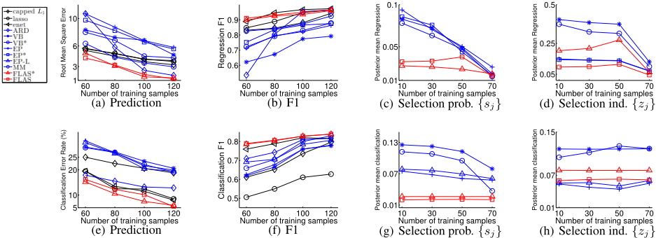
Results. Figures 1 a and e show the predictive performance of all the methods for regression and classification. FLAS* and FLAS show better performance than alternative methods, or at least comparable to them. Figures 1 b and f report the feature selection accuracy based on the F1 score, i.e., the harmonic average of the sensitivity and the specificity of the selected feature set. To compute the F1 score, we select features when the posterior mean of the selection indicators, E(zj), is over 0▷5 for Bayesian spike-and-slab models, or when model weights ♣wj♣ > 0▷001 for other methods. As we can see, FLAS* and FLAS achieve higher F1 scores for classification and comparable F1 score than the best alternatives in regression.
For selection uncertainty, we compare the posterior mean of sj and zj with the results of Gibbs sampling based on 100↪ 000 samples. We calculate the root mean square error to evaluate the difference from the ground truth and report the results in Figure 1 c, d, g, and h. It is clear that FLAS* and FLAS consistently obtain better or comparable uncertainty estimation to competing methods. This confirms the inference quality of our algorithm.
5.2 Large Real Benchmark Data sets
We then examine all the algorithms on 14 published large real datasets, including 8 classification datasets 3 and 6 regression datasets: Diffuse large B cell lymphoma (DLBCL) [Rosenwald et al., 2002], GSE5680 [Scheetz et al., 2006], Yearprediction 4 (Year), House-census 5 (House), 10K corpus [Kogan et al., 2009] and TIED 6 . Among the 14 datasets, the feature numbers are often at tens of thousands, while the sample sizes
1 www-stat.stanford.edu/⇠tibs/glmnet-matlab
2 www.public.asu.edu/⇠jye02/Software/GIST/
3 www.shi-zhong.com/software/docdata.zip
4 archive.ics.uci.edu/ml/datasets.html
5 www.cs.toronto.edu/⇠delve/data/census-house/desc.html
6 www.causality.inf.ethz.ch/repository.php
120
(g) Selection prob. ¶sj♦
(h) Selection ind. ¶zj♦
Figure 1: Simulation results, including the prediction accuracy, the F1 score of feature selection, and the root mean squared error for the posterior mean estimation of ¶sj♦ and ¶zj♦. Results are averaged over 50 runs.
| dataset | lasso | elast net | capped L1 | ARD | EP-L | FLAS* | FLAS |
|---|---|---|---|---|---|---|---|
| gse5680 | 0.107 ◦ 0.003 | 0.107 ◦ 0.003 | 0.107◦ 0.003 | 0.136 ◦ 0.005 | 0.72 ◦ 0.001 | 0.111 ◦ 0.002 | 0.089◦ 0.002 |
| 10k corpus | 0.382 ◦ 0.002 | 0.382 ◦ 0.002 | 0.382 ◦ 0.002 | 0.382 ◦ 0.384 | 0.385 ◦ 0.003 | 0.383 ◦ 0.003 | 0.372 ◦ 0.003 |
| tied | 0.656 ◦ 0.013 | 0.627 ◦ 0.014 | 0.656 ◦ 0.013 | 0.532 ◦ 0.017 | 1.11 ◦ 0.2 | 0.632 ◦ 0.017 | 0.656 ◦ 0.013 |
| House | 1.576 ◦ 0.011 | 1.578 ◦ 0.017 | 1.587 ◦ 0.012 | 0.435 ◦0.0006 | 0.430 ◦ 0.0002 | 0.441 ◦ 9.5e-4 | 0.425 ◦0.002 |
| Year | 0.296 ◦ 0.009 | 0.293 ◦ 0.007 | 0.307 ◦ 0.004 | 0.306 ◦ 0.006 | 0.32 ◦ 0.002 | 0.232◦ 5.04e-4 | 0.234 ◦ 0.0001 |
| dlbcl | 1.76 ◦ 0.026 | 1.75 ◦ 0.027 | 1.75 ◦ 0.028 | 2.38 ◦ 0.063 | 1.61 ◦ 0.050 | 1.56 ◦ 0.043 | 1.60◦ 0.047 |
| classic | 6.69 ◦ 0.002 | 5.94 ◦ 0.002 | 4.14 ◦ 0.002 | 18.2 ◦ 0.002 | 8.94 ◦ 0.002 | 4.2 ◦ 0.002 | 4.20 ◦ 0.001 |
| hitech | 23.2 ◦ 0.005 | 21.4 ◦ 0.004 | 21.3 ◦ 0.003 | 28.5 ◦ 0.019 | 25.2 ◦ 0.001 | 19.9 ◦ 0.002 | 19.9 ◦ 0.003 |
| k1b | 5.44 ◦ 0.005 | 4.91 ◦ 0.004 | 4.42 ◦ 0.004 | 23.0 ◦ 0.013 | 7.94 ◦ 0.004 | 4.73 ◦ 0.005 | 4.74 ◦ 0.005 |
| reviews | 7.68 ◦ 0.003 | 6.47 ◦ 0.002 | 6.09 ◦ 0.001 | 35.4 ◦ 0.05 | 8.28 ◦ 0.002 | 5.55 ◦ 0.001 | 5.54 ◦ 0.001 |
| sports | 3.72 ◦ 0.001 | 3.15 ◦ 0.0008 | 3.25 ◦ 0.0009 | 24.1 ◦ 0.032 | 10.9 ◦ 0.008 | 2.77 ◦0.0006 | 2.77 ◦0.007 |
| ng3sim | 19.3 ◦ 0.005 | 16.2 ◦ 0.003 | 15.4 ◦ 0.003 | 21.3 ◦ 0.006 | 14.5 ◦ 0.002 | 13.7 ◦ 0.002 | 13.6 ◦ 0.002 |
| ohscal | 13.8 ◦ 0.001 | 13.7 ◦ 0.001 | 13.8 ◦ 0.001 | 37.3 ◦ 0.02 | 13.7 ◦0.002 | 13.05 ◦ 0.001 | 13.1 ◦ 0.001 |
| la12 | 13.6 ◦ 0.002 | 12.5 ◦ 0.002 | 12.2 ◦ 0.002 | 30.1 ◦ 0.025 | 13.2 ◦ 0.002 | 11.04 ◦ 0.001 | 11.1 ◦ 0.001 |
are often at hundreds or thousands.
We compare our algorithms, FLAS* and FLAS, with lasso, elastic net, capped L1, ARD and EP-L. Note that we implement lasso and elastic net based on GIST, because the Glmnet software used in simulation is no longer feasible. We randomly split each dataset into two parts-10% samples for training and the rest for test-for 10 times and run all the methods on each partition. In each run, we use 10-fold cross validation on the training data to tune the free parameters. Table 1 lists the average prediction accuracy and standard errors on the original datasets. As we can see, in all datasets, except for Tied in regression, and classic and k1b in classification, our algorithms, FLAS* or FLAS, obtain smaller root mean square errors or classification error rates. We also examine the average training time of all the methods and it turns out that our approach spends less or comparable time than the others. For example, the running time in seconds on gse5680 and reviews are ¶lasso:2▷03, elastic net:2▷26, capped L1:15▷3, ARD:3▷52, EP-L: 6▷52, FLAS*:0.15, FLAS:0▷3♦, and ¶lasso:0▷32, elastic net:0▷29, capped L1:2▷3, ARD:26▷7, EP-L:1▷02, FLAS*:0▷25, FLAS:0.10♦ respectively.
6 Conclusion
We have presented a new scalable sparse Bayesian inference method for the spike-and-slab model. From a frequentist perspective, our approach is computationally efficient, and possesses oracle properties, and from a Bayesian point of view, it quantifies selection uncertainty. Our empirical results suggest that the spike and slab model can yield improved selection and predictive accuracy over the classical l1-type methods.
Acknowledgments
This work was supported by NSF CAREER award IIS1054903, and the Center for Science of Information, an NSF Science and Technology Center, under grant agreement CCF0939370.
@inproceedings{ijcai2016p267,
  title     = {Fast Laplace Approximation for Sparse Bayesian Spike and Slab Models},
  author    = {Naqvi, Syed Abbas Z. and Zhe, Shandian and Qi, Yuan and Yang, Yifan and Ye, Jieping},
  booktitle = {Proceedings of the Twenty-Fifth International Joint Conference on
               Artificial Intelligence, {IJCAI-16}},
  publisher = {AAAI Press / International Joint Conferences on Artificial Intelligence},
  editor    = {Subbarao Kambhampati},
  pages     = {1867--1972},
  year      = {2016},
  month     = {7},
  url       = {https://ijcai.org/proceedings/2016/267},
}
TY - CPAPER TI - Fast Laplace Approximation for Sparse Bayesian Spike and Slab Models AU - Naqvi, Syed Abbas Z. AU - Zhe, Shandian AU - Qi, Yuan AU - Yang, Yifan AU - Ye, Jieping T2 - Proceedings of the Twenty-Fifth International Joint Conference on Artificial Intelligence, IJCAI-16 PB - AAAI Press / International Joint Conferences on Artificial Intelligence PY - 2016 SP - 1867 EP - 1972 UR - https://ijcai.org/proceedings/2016/267 ER -Copied
Machine-readable versions of this paper, for tools and AI agents:





