
Parameter-Free Auto-Weighted Multiple Graph Learning: A Framework for Multiview Clustering and Semi-Supervised Classification
Proceedings of the Twenty-Fifth International Joint Conference on Artificial Intelligence. Pages 1881-1886.
Abstract
Graph-based approaches have been successful in unsupervised and semi-supervised learning. In this paper, we focus on the real-world applications where the same instance can be represented by multiple heterogeneous features. The key point of utilizing the graph-based knowledge to deal with this kind of data is to reasonably integrate the different representations and obtain the most consistent manifold with the real data distributions. In this paper, we propose a novel framework via the reformulation of the standard spectral learning model, which can be used for multiview clustering and semi-supervised tasks. Unlike other methods in the literature, the proposed method can learn an optimal weight for each graph automatically without introducing an additive parameter as previous methods do. Furthermore, our objective under semi-supervised learning is convex and the global optimal result will be obtained. Extensive empirical results on different real-world data sets demonstrate that the proposed method achieves comparable performance with the state-of-the-art approaches and can be used more practically.
- [Asuncion and Newman, 2007] Arthur Asuncion and David Newman. Uci machine learning repository, 2007.
- [Cai et al., 2011] Xiao Cai, Feiping Nie, Heng Huang, and Farhad Kamangar. Heterogeneous image feature integra- tion via multi-modal spectral clustering. In Computer Vision and Pattern Recognition (CVPR), 2011 IEEE Conference on, pages 1977-1984. IEEE, 2011.
- [Cai et al., 2013] Xiao Cai, Feiping Nie, Weidong Cai, and Heng Huang. Heterogeneous image features integration via multi- modal semi-supervised learning model. In Computer Vision (ICCV), 2013 IEEE International Conference on, pages 1737- 1744. IEEE, 2013.
- [Chaudhuri et al., 2009] Kamalika Chaudhuri, Sham M Kakade, Karen Livescu, and Karthik Sridharan. Multi-view clustering via canonical correlation analysis. In Proceedings of the 26th annual international conference on machine learning, pages 129-136. ACM, 2009.
- [Chua et al., 2009] Tat-Seng Chua, Jinhui Tang, Richang Hong, Haojie Li, Zhiping Luo, and Yantao Zheng. Nus-wide: a real- world web image database from national university of singa- pore. In Proceedings of the ACM international conference on image and video retrieval, page 48. ACM, 2009.
- [Hagen and Kahng, 1992] Lars Hagen and Andrew B Kahng. New spectral methods for ratio cut partitioning and clustering. Computer-aided design of integrated circuits and systems, ieee transactions on, 11(9):1074-1085, 1992.
- [Karasuyama and Mamitsuka, 2013] Masayuki Karasuyama and Hiroshi Mamitsuka. Multiple graph label propagation by sparse integration. Neural Networks and Learning Systems, IEEE Transactions on, 24(12):1999-2012, 2013.
- [Kumar et al., 2011] Abhishek Kumar, Piyush Rai, and Hal Daume. Co-regularized multi-view spectral clustering. In Advances in Neural Information Processing Systems, pages 1413-1421, 2011.
- [Lee and Grauman, 2009] Yong Jae Lee and Kristen Grauman. Foreground focus: Unsupervised learning from partially matching images. International Journal of Computer Vision, 85(2):143-166, 2009.
- [Li et al., 2015] Yeqing Li, Feiping Nie, Heng Huang, and Jun- zhou Huang. Large-scale multi-view spectral clustering via bipartite graph. In Proceedings of the Twenty-Ninth AAAI Con- ference on Artificial Intelligence, 2015.
- [Ng et al., 2002] Andrew Y Ng, Michael I Jordan, Yair Weiss, et al. On spectral clustering: Analysis and an algorithm. Ad- vances in neural information processing systems, 2:849-856, 2002.
- [Nie et al., 2010] Feiping Nie, Heng Huang, Xiao Cai, and Chris H Ding. Efficient and robust feature selection via joint `2,1 -norms minimization. In Advances in neural information processing systems, pages 1813-1821, 2010.
- [Nie et al., 2011] Feiping Nie, Zinan Zeng, Ivor W. Tsang, Dong Xu, and Changshui Zhang. Spectral embedded clustering: A framework for in-sample and out-of-sample spectral cluster- ing. IEEE Trans. Neural Networks, 22(11):1796-1808, 2011.
- [Nie et al., 2012] Feiping Nie, Dong Xu, and Xuelong Li. Ini- tialization independent clustering with actively self-training method. IEEE Trans. Systems, Man, and Cybernetics, Part B, 42(1):17-27, 2012.
- [Nie et al., 2014] Feiping Nie, Xiaoqian Wang, and Heng Huang. Clustering and projected clustering with adaptive neighbors. In The 20th ACM SIGKDD International Confer- ence on Knowledge Discovery and Data Mining, KDD '14, New York, NY, USA -August 24 -27, 2014, pages 977-986, 2014.
- [Nie et al., 2016] Feiping Nie, Xiaoqian Wang, Michael I Jor- dan, and Heng Huang. The constrained laplacian rank algo- rithm for graph-based clustering. 2016.
- [Niu et al., 2010] Donglin Niu, Jennifer G Dy, and Michael I Jordan. Multiple non-redundant spectral clustering views. In Proceedings of the 27th international conference on machine learning (ICML-10), pages 831-838, 2010.
- [Shi and Malik, 2000] Jianbo Shi and Jitendra Malik. Normal- ized cuts and image segmentation. Pattern Analysis and Machine Intelligence, IEEE Transactions on, 22(8):888-905, 2000.
- [Von Luxburg, 2007] Ulrike Von Luxburg. A tutorial on spectral clustering. Statistics and computing, 17(4):395-416, 2007.
- [Wang et al., 2009] Meng Wang, Xian-Sheng Hua, Richang Hong, Jinhui Tang, Guo-Jun Qi, and Yan Song. Unified video annotation via multigraph learning. Circuits and Sys- tems for Video Technology, IEEE Transactions on, 19(5):733- 746, 2009.
- [Winn and Jojic, 2005] John M. Winn and Nebojsa Jojic. LO- CUS: learning object classes with unsupervised segmentation. In 10th IEEE International Conference on Computer Vision (ICCV 2005), 17-20 October 2005, Beijing, China, pages 756- 763, 2005.
- [Xia et al., 2010] Tian Xia, Dacheng Tao, Tao Mei, and Yong- dong Zhang. Multiview spectral embedding. Systems, Man, and Cybernetics, Part B: Cybernetics, IEEE Transactions on, 40(6):1438-1446, 2010.
- [Yu et al., 2012] Jun Yu, Meng Wang, and Dacheng Tao. Semisupervised multiview distance metric learning for car- toon synthesis. Image Processing, IEEE Transactions on, 21(11):4636-4648, 2012.
- [Zhu et al., 2003] Xiaojin Zhu, Zoubin Ghahramani, John Laf- ferty, et al. Semi-supervised learning using gaussian fields and harmonic functions. In ICML, volume 3, pages 912-919, 2003.
References were extracted automatically from the PDF and may contain errors.
Full text extracted automatically from the PDF; figures, tables and equations may differ. The PDF is the version of record.
1 Introduction
Graph-based learning provides an efficient approach for modeling data in clustering and classification problems. Since it works with a constructed graph, different measurements and insights can be built up subsequently, such as the relations between unlabeled data (clustering) or from labeled to unlabeled data (semi-supervised classification). Practically, many applications involve data obtained from different views, and multiple graphs need to be built. It is often assumed that each individual graph captures the partial information but they all admit the same underlying clustering of the data. Thus, the main challenge of this problem is how to effectively integrate these graphs in specific tasks.
Among the numerous clustering methods, the use of manifold information in spectral clustering method has achieved the state-of-the-art performance. Many works have been summarized in [Von Luxburg, 2007], such as ratio cut [Hagen and Kahng, 1992], normalized cut [Shi and Malik, 2000]. Some other works clustered data in high dimension [Nie et al., 2011] or construct the data similarity matrix by adaptively selecting more reliable neighbors [Nie et al., 2014]. When accessing to multi-view data, some researches based on multiple graph learning have been developed. [Chaudhuri et al., 2009] projected the data into a lower dimensional subspace and clustered multiview data via canonical correlation analysis. [Niu et al., 2010] learned non-redundant subspaces that provide multiple clustering solutions to the original problem. To keep the consistency to the same clustering across all of graphs, [Kumar et al., 2011] appealed to a co-regularization framework to acquire the final clustering hypotheses. A similar approach integrating heterogenous image features with graphs was proposed for image clustering in [Cai et al., 2011]. This kind of methods fail to differ the reliability of different views and are prone to be ruined by a weak one. Thus, some methods [Xia et al., 2010; Li et al., 2015] adaptively learn a weight for each graph during the optimization.
On the other hand, the graph-based learning can be modeled as a transductive semi-supervised classification method, Given a data set which is partially labeled, the unlabeled ones can be labeled according to learning the pairwise similarity. Hence, it is also called label propagation. One of the typical representative works was proposed by [Zhu et al., 2003], which explicitly compute the label vectors for unlabeled samples. By actively selecting training set, [Nie et al., 2012] presented a initialization independent method. For multiple graph learning in semi-supervised classifications, many applications in computer vision, such as video annotation [Wang et al., 2009], cartoon synthesis [Yu et al., 2012] and image classification [Cai et al., 2013], have achieved good predictive performance. In view of that many approaches can only give nonzero weights to every graph, [Karasuyama and Mamitsuka, 2013] proposed another multiple graph learning method, where the weights can be sparse.
Although all above unsupervised clustering methods and semi-supervised classification techniques have achieved good performance, some of them ignore the diversity of graphs and others learn a weight for each graph with an additional parameter. In this paper, following the assumption that all the graphs share the same underlying clustering but each individual contains the incomplete information to learn the real manifold, we propose a novel Auto-weighted Multiple Graph Learning (AMGL) framework to learn a set of weights automatically for all the graphs and this process does not need any parameter. This new AMGL framework can be applied both to multiview clustering and semi-supervised classification tasks. What's more, AMGL models a convex problem when it is applied in semi-supervised learning. We design an efficient algorithm to optimize the proposed problem. The experimental results on different data sets demonstrate that our methods have comparable results with the state-of-the-art methods.
2 ProblemFormulation
In this section, we first revisit the basic form of graph-based spectral clustering and semi-supervised learning, and then summarize the traditional multiple graph learning methods into two general forms. By analyzing the deficiencies of them, we finally propose a new framework.
2.1 Background andMotivation
Let X = [x1↪ ▷▷▷↪ xn]T 2 Rn⇥d denote data matrix, where n is the number of data points and d is the dimension of feature. Given the whole data set X, the adjacent matrix W = ¶wij♦ 2 Rn⇥n ↪ 8i↪ j 2 1↪ ▷▷▷↪ n and the corresponding degree matrix D (dii = Pnj=1 wij) can be constructed. We define the cluster indicator matrix F = [f1↪ ▷▷▷↪ fn]T 2 Rn⇥c , where c is the number of classes. Therefore, the classical Ratio Cut clustering can be written as
and the Normalized Cut can be represented by
where L = D -W is a so-called Laplacian matrix. Both Eq. (1) and Eq. (2) can be solved by eigenvalues calculating. When only l (l < n) samples are labeled in the raw data (Without loss of generality, we rearrange all the samples and let the front l samples be labeled), it becomes a transductive semi-supervised learning problem, which can be written as
blocks after the l-th row and column: L = Lll Llu
Lul Luu ].
where yi is the given indicator vector for the i-th sample. If i-th sample belongs to j-th class, we have yij = 1 and other elements in yi are all 0s. We split Laplacian matrix L into four
Let F = [Fl; Fu] and the constraint in problem (3) can be written as Fl = Yl where Yl = [y1↪ ▷▷▷↪ yl]T . According to [Zhu et al., 2003], the solution of problem (3) can be directly given as
For simplicity, we use C to denote different constraints in Eq. (1), Eq. (2) and Eq. (3) and obtain a unified form:
For multi-view data, let m be the number of views and X(1) ↪ ▷▷▷↪ X(m) be the data matrix of each view, where X(v) 2 Rn⇥d(v) for v = 1↪ ▷▷▷↪m and d(v) is the feature dimension of v-th view. For each single view, a normalized Laplacian matrix is constructed, so we have L(1) ↪ ▷▷▷↪L(m) 2 Rn⇥n . A simple and direct way to use these graphs is to stack up to a new one and put it into the standard spectral analysis model. However, this strategy neglects the importance of different graphs and may suffer when an unreliable graph is added to. A more reasonable approach is to linearly combine these different graphs with suitable weights θ(v) (v = 1↪ ▷▷▷↪m), and keep the smooth of the weights distribution by resorting to an extra parameter γ. We constrain the indicator matrix F to be a unified one across all the views and set aside the normalization to different graphs. Thus, this thought can be modeled as the following problem
which is introduced in [Xia et al., 2010; Cai et al., 2013; Li et al., 2015]. A similar form applied in [Karasuyama and Mamitsuka, 2013] is
where θ = ⇥θ(1) ↪ ▷▷▷↪ θ(m) ⇤. In Eq. (6), γ is set to a value greater than 1, while in Eq. (7), γ is set to a non-negative value. As shown in our experiments (see Section 5.2), for Eq. (6) and Eq. (7), the choice of γ is crucial to the final performance and its optimal value changes for different data sets. Thus, our goal is to remove such a parameter while preserving the good performance.
2.2 Auto-weightedMultiple Graph Learning
In this paper, we propose a new general framework for multiple graph learning with the following form
where no weight factors are explicitly defined. The Lagrange function of problem (8) can be written as
where ⇤ is the Lagrange multiplier, G(⇤↪ F ) is the formalized term derived from the constraints. Taking the derivative of Eq. (9) w.r.t F and setting the derivative to zero, we have
where
Note that in Eq. (11), ↵(v) is dependent on the target variable F and Eq. (10) can not be directly solved. But if ↵(v) is set to be stationary, Eq. (10) can be considered as the solution to the following problem
which looks simpler to be solved. Supposing that F can be calculated from Eq. (12), this F will be continuously used to update ↵(v) according to Eq. (11), which inspires us to take an alternating optimization strategy to compute F and ↵(v) iteratively. We summarize this process in Alg. 1. Since Alg. 2 and Alg. 3 have the same initialization with Alg. 1, we will not show it any more.
Algorithm 1 The general algorithm of AMGL
Input: Data for m views ¶X(1) ↪ ▷▷▷↪X(m) ♦ and X(v) 2 Rn⇥dv , number of classes c Initialize the weight factor ↵(v) = 1m for each view; Compute Laplacian matrix L(v) for each view; Calculate L = Pmv=1 ↵(v)L(v) repeat
- Compute F by solving Eq. (12)
- Update ↵(v) by Eq. (11)
until converge
Subsequent operations to indicator matrix F
Output: The label of each unlabeled data point
So far, based on above analysis, some significant conclusions can be drawn:
- Supposing that this alternating optimization converges (it will be proved in Section 4.1) and b F denotes the converged value of F, according to Eq. (10) and Eq .(11), F is at least a local optimal solution to Eq. (8).
- b 2. Let b↵(v) be the value of ↵(v) after optimization, according to Eq. (12), it is exactly the linear combination of different graphs using the learned weights b↵(v) . Comparing with Eq. (6) and Eq. (7), Eq. (12) is the real problem we want to solve and this is the core why we consider solving such a problem like Eq. (8).
- Unlike Eq.(5) and Eq. (6), which learn the weights depending on an extra parameter, the proposed framework has no parameter to handle and naturally learns the view weights and the target indicator matrix simultaneously.
- If view v is good, then Tr (F T L(v)F ) should be small, and thus the learned weight ↵(v) for view v is large according to Eq.(11). Accordingly, a bad view will be assigned a small weight. That is to say, our method optimizes the weights meaningfully and can obtain better result than the classical combination approach which assigns equal weight to all the views.
3 AMGL for Clustering and Semi-supervised Classification
For simplicity, we take the unnormalized Laplacian matrix in the following statement. Seeing that AMGL conducts a two-variable alternating optimization process and the main steps have been given in Alg. 1, we only show the essential analyses.
3.1 AMGL for Clustering
In spectral clustering, it is known that the indicator F must satisfy the following constraint
Substituting this constraint function in Eq. (8), we obtain the following objective for multi-view clustering:
Based on Alg. 1, the problem (14) can be solved by an iterative algorithm as described in Alg. 2.
Algorithm 2 The algorithm of AMGL for clustering
Input: Data for m views ¶X(1) ↪ ▷▷▷↪X(m) ♦ and X(v) 2 Rn⇥dv , number of classes c
repeat
1. Compute F by using Eq. (12) with calculating the 2 to c + 1 smallest eigenvalues of eL = Pmv=1 ↵(v)L(v) . 2. Update ↵(v) by Eq. (11)
until converge
Treat each row of F as a new representation of each data point and compute the clustering labels by using k-means algorithm.
Output: Cluster label of each data point
3.2 AMGL for Semi-supervised Classification
For semi-supervised classification, suppose there are l(1 l < n) data points labeled, we rearrange them as before and have the following constraints
Taking this constraint into Eq. (8), we can formulate the semisupervised classification problem as
and our goal is to obtain the fi (i = l + 1↪ ▷▷▷↪ n) for unlabeled data. Following the optimization in Alg. 1, when we fix ↵ and update F , Eq. (16) can be written as
where eL = Pmv=1 ↵(v)L(v) . Referring to Eq. (4), we can directly give the solution to Eq. (17) as
Fu = -eLuu eLulYl↪
where Fu, eLuu, eLul and Yl are consistent with Eq. (4). Different from clustering, we resort to the following equation to get the label vector yi for the unlabeled data point (we assign 1 to the j-th element and 0 to others):
The complete algorithm can be summarized in Alg. 3.
Algorithm 3 The algorithm of AMGL for semi-supervised classification
Input: Data for m views ¶X(1) ↪ ▷▷▷↪X(m) ♦ and X(v) 2 Rn⇥dv , the labels for the l labeled data Yl
repeat
1. Calculate Fu by using Eq. (18)
2. Let F = [Yl; Fu] and update ↵(v) by Eq. (11)
until converge
Assign the single class label to unlabeled data by Eq. (19)
Output: The predicted labels for the unlabeled data
4 Theoretical Analysis
In this section, we first prove the convergence of the Alg. 1, which naturally engages for the convergence Alg. 2 and Alg. 3. Furthermore, we present in semi-supervised classification, the problem (16) is convex and the global optimal solution will be obtained.
4.1 Convergence Analysis
To prove the convergence of the Alg. 1, we need the following lemma introduced in [Nie et al., 2010]:
Lemma 1 For any positive number a and b, the following inequality holds:
Theorem 1 Each updated F in Alg. 1 will monotonically decease the objective of the problem (8) in each iteration, which makes the solution converge to a local optimum of the problem (8).
Proof: We use e F to denote the updated F in each iteration. According to the optimization to F in Alg. 1, we know that e F makes the objective of Eq. (12) have the smaller value than F . Combining ↵(v) = 1.⇣2qT r (F T L(v)F )⌘, we can derive:
According to Lemma 1, we have
Summing Eq. (21) and Eq. (22) in the two sides, we arrive at
Thus the alternating optimization will monotonically decrease the objective of the problem (8) in each iteration until it converges. In the convergence, the equality in Eq. (23) holds, thus e F will satisfy Eq. (10), the KKT condition of problem (8). Therefore, the Alg. 1 will converge to a local optimum of the problem (8).
4.2 Convex of Problem (16)
To prove the convex of problem (16), we introduce the following lemma.
Lemma 2 For any arbitrary convex function h (x) and linear function g (x), the compound function h (g (x)) is convex.
Proof: For any real number ↵ and β, because g (x) is a linear function and h (x) is convex, we have
h (g (↵x+βy)) = h (↵g (x) +βg (y)) ↵h (g (x)) +βh (g (y)) ▷ (24)
Obviously, the compound function h (g (x)) is convex.
For indicator matrix F 2 Rn⇥c , we define f T = [f11↪ ▷▷▷↪ fn1↪ f12↪ ▷▷▷↪ fn2↪ ▷▷▷↪ f1c↪ ▷▷▷↪ fnc]. It is easily verified that the following equation holds:
where A(v) 2 Rnc⇥nc is a block diagonal matrix and each non-zero block equals to L(v) . Obviously, A(v) is positive semi-define since L(v) is positive semi-define. Therefore, there must exist a matrix B(v) 2 Rnc⇥p(v) (p(v) is the rank of L(v) ) that satisfies
Taking Eq. (26) into the root form of the left side in Eq. (25), we can obtain
Because k▷k2 is a convex and (B(v) )T f is a linear function w.r.t x, it can be concluded that the objective of Eq. (16) is convex according to Lemma 2. Since the constraints in Eq. (16) are linear functions, we know that problem (16) is convex. Combining Theorem 1 we conclude that Alg. 3 will obtain the global optimal solution to the problem (16).
5 Experiment
In this paper, a new graph construction approach introduced in [Nie et al., 2016] is adopted in our methods. The advantage of this approach is that it has no parameters if we set the number of neighbors.We evaluate the performance of the proposed framework AMGL for clustering and semi-supervised classification on the following four data sets:
MSRC-v1 data set [Winn and Jojic, 2005] contains 240 images and can be divided into 8 classes. Following [Lee and Grauman, 2009], we select 7 classes composed of tree, building, airplane, cow, face,car, bicycle and each class has 30 images. To distinguish all of scenes, we extract five visual features from each image: 24 Color Moment, 576 Histogram of Oriented Gradient, 512 GIST, 256 Local Binary Pattern and 254 Centrist features.
Handwritten numerals data set [Asuncion and Newman, 2007] is composed of 2,000 data points for 0 to 9 ten digit classes and each class has 200 data points. Six published features can be used for classification: 76 Fourier coefficients of the character shapes (FOU), 216 profile correlations (FAC), 64 Karhunen-love coefficients (KAR), 240 pixel averages in 2 ⇥ 3 windows (PIX), 47 Zernike moment (ZER) and morphological (MOR) features.
CiteSeer data set [Asuncion and Newman, 2007] consists of 3,312 documents which are about scientific publications. These documents can be further classified into 6 classes: Agents, AI, DB, IR, ML and HCI. For our multi-view learning classifications, a 3,703-dimensional vector representing whether the key words are included for the text view, and the other 3279-dimensional vector that records the citing relations between every two documents are built up.
NUS-WIDE data set [Chua et al., 2009] contains 269,648 images of 81 concepts. In our experiments, 12 categories about animal concept are selected. They are cat, cow, dog, elk, hawk, horse, lion, squirrel, tiger, whales, wolf, and zebra. Each image can be represented by six type low-level features: 64 color histogram, 144 color correlogram, 73 edge direction histogram, 128 wavelet texture, 225 block-wise color moment and 500 bag of words based on SIFT descriptions.
5.1 Performance Evaluation
Although the proposed approach has no free parameter, we allow the compared methods to tune the parameter γ (if has) with the strategy that γ for the type of Eq. (5) is searched in logarithm form (log10γ from 0.1 to 2 with step size 0.2) while it is a little different (log10γ from -5 to 5 with step size 1) for the type of Eq. (6). In addition, if there are other parameters in compared methods, they will be set as the optimal values. We construct each graph by selecting 5-nearest neighbors among raw data. Both an unnormalized and normalized Laplacian matrix will be computed for each method and the better result will be employed in the final performance comparison. All the experiments are repeated for 20 times and the average results are reported. We mark the best result in bold face.
Clustering Evaluation
Besides conducting each single view for Spectral Clustering (SC) [Ng et al., 2002], the proposed method is compared with some state-of-the-art approaches: Co-regularized Spectral Clustering(CoregSC) [Kumar et al., 2011], Multi-Modal Spectral Clustering (MMSC) [Cai et al., 2011] and Multiview Spectral Clustering (MVSC) [Li et al., 2015]. For experimental results, two metrics mean purity and normalized mutual information (NMI) are employed.
| Data set | MSRC-v1 | HW | CiteSeer | NUS |
|---|---|---|---|---|
| SC(1) | 39.52 | 58.95 | 18.75 | 16.29 |
| SC(2) | 58.10 | 83.10 | 21.75 | 19.83 |
| SC(3) | 69.05 | 72.15 | - | 17.54 |
| SC(4) | 48.10 | 72.35 | - | 20.38 |
| SC(5) | 56.19 | 55.25 | - | 17.11 |
| SC(6) | - | 53.25 | - | 18.50 |
| CoregSC | 69.04 | 82.23 | 20.38 | 24.20 |
| MMSC | 77.14 | 85.35 | 22.50 | 26.67 |
| MVSC | 81.45 | 86.05 | 22.56 | 28.03 |
| AMGL | 79.09 | 85.92 | 21.92 | 25.08 |
| Data set | MSRC-v1 | HW | CiteSeer | NUS |
| SC(1) | 0.2850 | 0.5758 | 0.0206 | 0.0604 |
| SC(2) | 0.4763 | 0.8187 | 0.0589 | 0.0840 |
| SC(3) | 0.6383 | 0.7190 | - | 0.0573 |
| SC(4) | 0.3982 | 0.7213 | - | 0.0876 |
| SC(5) | 0.4692 | 0.5384 | - | 0.0681 |
| SC(6) | - | 0.5286 | - | 0.0808 |
| CoregSC | 0.6754 | 0.8068 | 0.0540 | 0.1105 |
| MMSC | 0.7357 | 0.8460 | 0.0600 | 0.1315 |
| MVSC | 0.7197 | 0.8585 | 0.0558 | 0.1600 |
| AMGL | 0.7432 | 0.8515 | 0.0469 | 0.1229 |
Table 1 and Table 2 show the clustering purity and NMI respectively. In general, almost every multiple graph-based clustering method obtains the better result than single graph learning result. Furthermore, AMGL constantly outperforms the best single graph learning result and achieves a comparable or even superior result to other methods. As we know, AMGL has no extra parameter to handle and automatically learns the weight for each graph. Thus, comparing with the previous works, our method is convenient to use and shows strong practicability in multi-view clustering.
Semi-supervised Classification
On different proportions of labeled data (denoted with ⌧), we investigate the single graph leaning of Label Propagation (LP) [Zhu et al., 2003] and compare our method with some popular multiple graph leaning methods for semi-supervised classification: Sparse Multiple Graph Integration (SMGI) [Karasuyama and Mamitsuka, 2013], and Adaptive MultiModel Semi-Supervised classification (AMMSS) [Cai et al., 2013].
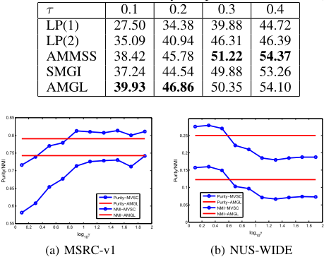
Table 3 and Table 4 show the semi-supervised classification performance on four data sets. In general, almost all of the multiple graph learning methods outperform the best single graph learning of label propagation. Comparing with the state-of-the-art approaches, our method keeps a close result to the best performance, such as in Handwritten numerals and NUS-WIDE data sets, and sometimes even achieves the best performance, especially in CiteSeer data set.
| Data set | MSRC-v1(%) | Handwritten numerals(%) | NUS-WIDE(%) | |||||||||
|---|---|---|---|---|---|---|---|---|---|---|---|---|
| ⌧ | 0.1 | 0.2 | 0.3 | 0.4 | 0.1 | 0.2 | 0.3 | 0.4 | 0.1 | 0.2 | 0.3 | 0.4 |
| LP(1) | 39.15 | 45.24 | 49.66 | 48.41 | 81.83 | 82.59 | 83.37 | 83.52 | 19.77 | 20.89 | 22.14 | 22.36 |
| LP(2) | 69.84 | 80.95 | 81.75 | 82.14 | 92.79 | 93.75 | 94.07 | 94.57 | 24.72 | 24.53 | 26.13 | 26.39 |
| LP(3) | 77.78 | 85.12 | 88.10 | 89.12 | 94.39 | 96.72 | 97.03 | 97.39 | 17.13 | 17.14 | 16.31 | 17.64 |
| LP(4) | 60.32 | 69.05 | 72.22 | 74.15 | 93.78 | 96.48 | 97.61 | 97.63 | 21.99 | 24.48 | 23.93 | 16.39 |
| LP(5) | 67.72 | 72.79 | 73.81 | 75.40 | 82.98 | 83.05 | 82.78 | 82.52 | 22.87 | 27.71 | 27.44 | 28.75 |
| LP(6) | - | - | - | - | 41.12 | 41.51 | 43.05 | 44.27 | 24.44 | 25.26 | 26.73 | 27.57 |
| AMMSS | 83.41 | 88.28 | 89.35 | 91.67 | 96.78 | 97.13 | 97.21 | 97.83 | 30.56 | 35.84 | 39.21 | 40.89 |
| SMGI | 83.02 | 89.88 | 88.84 | 90.48 | 94.07 | 96.75 | 97.75 | 98.33 | 31.03 | 35.24 | 38.09 | 40.60 |
| AMGL | 82.46 | 87.50 | 89.90 | 91.47 | 94.78 | 96.18 | 97.37 | 97.75 | 28.93 | 33.59 | 36.43 | 38.28 |
| ⌧ | 0.1 | 0.2 | 0.3 | 0.4 |
|---|---|---|---|---|
| LP(1) | 27.50 | 34.38 | 39.88 | 44.72 |
| LP(2) | 35.09 | 40.94 | 46.31 | 46.39 |
| AMMSS | 38.42 | 45.78 | 51.22 | 54.37 |
| SMGI | 37.24 | 44.54 | 49.88 | 53.26 |
| AMGL | 39.93 | 46.86 | 50.35 | 54.10 |
5.2 Why AMGL
In this part, we further exploit the property of the proposed methods. According to the statement in Section 2.1, Eq. (7) is often used to model a semi-supervised problem [Karasuyama and Mamitsuka, 2013] while the type of Eq. (6) can be applied both in clustering [Li et al., 2015] and semisupervised classification [Cai et al., 2013]. Thus, we compare our method with MVSC in clustering, with AMMSS and SMGI under semi-supervised classification. For simplicity, we analyze the experimental results on MSRC-v1 and NUSWIDE data sets.
From Figure 1, it is observed that for the optimal γ, mean purity and NMI of MVSC are better than our method, but its performance drops down dramatically with the change of γ. In addition, comparing Figure 1(a) with Figure 1(b), we note that MVSC obtains the best performance at the different γ in two data sets. For MSRC-v1, it seems a larger γ is more suitable, while for NUS-WIDE, a smaller γ is preferred. In semi-supervised classification, where ⌧ = 0▷2, from Figure 2 the similar conclusions can be come to. For AMMSS and SMGI, they enjoy the good performance at the optimal γ but are prone to get a terrible result when γ changes. Furthermore, from a data set to another one, the parameter γ needs to be tuned anew, which makes attempting to apply a fixed γ throughout all the applications is not available in practice.
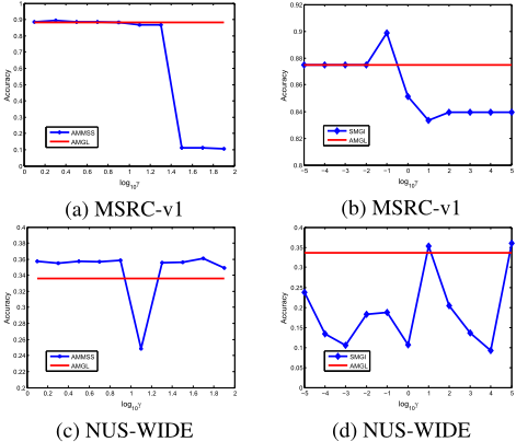
Particularly, in clustering and semi-supervised learning, there are few labeled data and thus the traditional supervised hyperparameter tuning techniques such as cross validation can not be used. Therefore, a method, such like the proposed approach, without too much accuracy loss but having no free parameter, is interesting and acceptable.
6 Conclusion
In this paper, we propose a novel parameter-free autoweighted multiple graph learning framework, named AMGL. This model can be used both for multiview clustering and semi-supervised classification. The proposed methods have no parameter to deal with and can naturally assign suitable weights to all of the graphs. The relative proof guarantees that the proposed framework can converge to a local optimal solution. Particularly, when it is applied to semi-supervised classification, we find that the corresponding problem becomes convex and the global optimal solution will be obtained after optimization. Experimental results on four data sets show the proposed methods have the comparable or even better accuracy than the state-of-the-art methods.
Acknowledgments
This work is supported by the Fundamental Research Funds for the Central Universities (Grant no. 3102015BJ(II)JJZ01).
@inproceedings{ijcai2016p269,
  title     = {Parameter-Free Auto-Weighted Multiple Graph Learning: A Framework for Multiview Clustering and Semi-Supervised Classification},
  author    = {Nie, Feiping and Li, Jing and Li, Xuelong},
  booktitle = {Proceedings of the Twenty-Fifth International Joint Conference on
               Artificial Intelligence, {IJCAI-16}},
  publisher = {AAAI Press / International Joint Conferences on Artificial Intelligence},
  editor    = {Subbarao Kambhampati},
  pages     = {1881--1886},
  year      = {2016},
  month     = {7},
  url       = {https://ijcai.org/proceedings/2016/269},
}
TY - CPAPER TI - Parameter-Free Auto-Weighted Multiple Graph Learning: A Framework for Multiview Clustering and Semi-Supervised Classification AU - Nie, Feiping AU - Li, Jing AU - Li, Xuelong T2 - Proceedings of the Twenty-Fifth International Joint Conference on Artificial Intelligence, IJCAI-16 PB - AAAI Press / International Joint Conferences on Artificial Intelligence PY - 2016 SP - 1881 EP - 1886 UR - https://ijcai.org/proceedings/2016/269 ER -Copied
Machine-readable versions of this paper, for tools and AI agents:





