Parallel Pareto Optimization for Subset Selection

1 Introduction

Given a total set of n variables, the subset selection problem is to select a subset of size at most k for optimizing some given objective. One origin of this problem is the column subset selection problem [Gu and Eisenstat, 1996], which aims at selecting a few columns from a matrix that capture as much of the matrix as possible. Since then, subset selection has been significantly extended and numerous applications of it have emerged, e.g., feature selection, sparse learning, compressed sensing, etc.

Subset selection is NP-hard in general [Davis et al., 1997]. Much effort has been put into developing polynomial-time approximation algorithms. These algorithms can be mainly categorized into two branches, greedy algorithms and convex relaxation methods. Greedy algorithms iteratively add or remove one variable that makes the given objective currently optimized [Gilbert et al., 2003; Tropp, 2004]. Albeit widely used in practice, the performance of these algorithms is limited due to their greedy nature. Convex relaxation methods relax the original problem by replacing the set size constraint (i.e., the `0-norm constraint) with convex constraints, e.g., the `1-norm constraint [Tibshirani, 1996] and the elastic net penalty [Zou and Hastie, 2005]. However, the optimal solutions of the relaxed problem could be distant to that of the original problem.

⇤This work was supported by the NSFC (61333014, 61375061, 61329302), the Collaborative Innovation Center of Novel Software Technology and Industrialization, and the 2015 Microsoft Research Asia Collaborative Research Program.

Recently, Pareto optimization has been shown to be very powerful for the subset selection problem [Qian et al., 2015c]. The Pareto Optimization for Subset Selection (POSS) method treats subset selection as a bi-objective optimization problem, which requires optimizing the given objective and minimizing the subset size simultaneously. Then, a bi-objective evolutionary algorithm with theoretical guarantee [Yu et al., 2012; Qian et al., 2015a; 2015b] is applied to solve it. Finally, the best solution satisfying the size constraint is picked out from the solution set produced by POSS. POSS is proved to achieve the best previous known polynomial-time approximation guarantee [Das and Kempe, 2011] on the sparse regression problem [Miller, 2002], a representative example of subset selection. Particularly, it can also even find an optimal solution on an important subclass of sparse regression [Das and Kempe, 2008]. In addition to the theoretical guarantee, POSS has also achieved significantly better empirical performance than the greedy and the relaxation methods.

POSS requires calling 2ek2n (e ⇡ 2▷71828 is Euler's number) number of objective function evaluations [Qian et al., 2015c] to achieve a high quality solution, which could be unsatisfactory from the practical viewpoint when k and n are large. On the other hand, POSS is a sequential algorithm that cannot be readily parallelized, which hinders the exploration of modern computer facilities for applying POSS to largescale real-world problems.

In this paper, we propose a parallel version of POSS, called PPOSS. Instead of generating one solution at a time (as in POSS), PPOSS generates as many solutions as the number of processors at a time, and can be easily parallelized. More important, on subset selection with monotone objective functions, we prove that, while preserving the solution quality,

(1) when the number of processors is limited (less than the number n of variables), the running time of PPOSS can be reduced almost linearly w.r.t. the number of processors;

(2) with increasing number of processors, the running time can be continuously reduced, eventually to a constant.

We further show that the obtained approximation quality reaches the best previous known approximation bound on two well-known instances in the studied class: any submodular objective function and sparse regression with a specific non-submodular objective function. Experimental results on sparse regression tasks verify our theoretical analysis, and suggest that the asynchronous implementation of PPOSS is more efficient, while introduces little loss in solution quality.

The rest of the paper is organized as follows. Section 2 introduces the subset selection problem and the POSS method. In Section 3, we propose the PPOSS method and give the theoretical analysis. Section 4 presents the empirical studies. Section 5 concludes this paper.

2 Subset Selection

The subset selection problem as presented in Definition 1 is to select a subset S from a total set V of variables such that a given objective f is minimized with the constraint ♣S♣  k, where ♣ · ♣ denotes the size of a set. It is generally NPhard [Natarajan, 1995; Davis et al., 1997]. Note that we only consider minimization since maximizing f is equivalent to minimizing -f .

Definition 1 (Subset Selection). Given all variables V = ¶X1↪ ▷ ▷ ▷ ↪Xn♦, an objective f and a positive integer k, it is to find a set of at most k variables minimizing f, i.e.,

Sparse regression [Miller, 2002] as presented in Definition 2 is an example of subset selection. It is to find a sparse solution to the linear regression problem. Note that we do not distinguish between S and its index set IS = ¶i ♣ Xi 2 S♦ for notational convenience, and we assume that all variables are normalized to have expectation 0 and variance 1.

Definition 2 (Sparse Regression). Given all observation variables V = ¶X1↪ ▷ ▷ ▷ ↪Xn♦, a predictor variable Z and a positive integer k, define the mean squared error of a subset S ✓ V as

Sparse regression is to find a set of at most k variables minimizing the mean squared error, i.e.,

In the previous theoretical analysis for sparse regression [Das and Kempe, 2008; 2011; Qian et al., 2015c], an equivalent form is often used

where R2Z↪S = (V ar(Z)-MSEZ↪S)◁V ar(Z) is the squared multiple correlation [Diekhoff, 1992; Johnson and Wichern, 2007], and can be simplified to be 1 - MSEZ↪S, because Z is assumed to be normalized to have variance 1 (i.e., V ar(Z) = 1). Das and Kempe [2011] proved that the greedy algorithm achieves the best known approximation guarantee. The greedy algorithm iteratively adds one variable with the largest R2 improvement until k variables are selected. It can produce a subset S with R2Z↪S ≥ (1 - e-γ ) · OPT, where OPT denotes the optimal function value of Eq. (2) and γ is the submodularity ratio [Das and Kempe, 2011].

2.1 The POSSMethod

Qian et al. [2015c] proposed a Pareto optimization method for subset selection, called POSS. Let a binary vector s 2 ¶0↪ 1♦n represent a subset S of V , where si = 1 if the variable Xi is in S and si = 0 otherwise. Note that s 2 ¶0↪ 1♦n and its corresponding subset will not be distinguished for notational convenience. The POSS method reformulates the original problem Eq. (1) as a bi-objective minimization problem

where

That is, POSS minimizes the original objective and the subset size simultaneously. Note that setting f1 to +1 is to exclude trivial or overly bad solutions.

For comparing solutions in the bi-objective setting, both the two objective values need to be compared. For two solutions s and s0 , s weakly dominates s0 (i.e., s is better than s0 , denoted as s ⪯ s0 ) if f1(s)  f1(s0 ) ^ f2(s)  f2(s0 ) (i.e., s has a smaller or equal value on both the objectives); s dominates s0 (i.e., s is strictly better, denoted as s ≺ s0 ) if s ⪯ s0 and either f1(s) < f1(s0 ) or f2(s) < f2(s0 ) (i.e., s has a strictly smaller value on one objective, and meanwhile has a smaller or equal value on the other objective). The domination relationship can be formally stated as follows:

But if both s is not better than s0 and s0 is not better than s, they are incomparable. Note that an isolation function I : ¶0↪ 1♦n ! R was further introduced in [Qian et al., 2015c] to determine if two solutions are allowed to be compared. However, I is set to be a constant function in this paper, and it can be just ignored because every solution has the same I value.

The procedure of POSS is described in Algorithm 1. It starts from the solution representing an empty set (line 1) and then iteratively tries to improve the solutions in the archive P (lines 3-12). In each iteration, a new solution s0 is generated by randomly flipping bits of an archived solution s selected from the current P (lines 4-5); its two objective values are then evaluated (line 6); if s0 is not strictly worse than any previously archived solution (line 7), it will be added into P , and meanwhile those previously archived solutions worse than s0 will be removed from P (lines 8-9). After T iterations, the best solution (i.e., having the smallest f1 value) satisfying the size constraint in P is selected (line 13).

For sparse regression, POSS using E[T]  2ek2n and a constant isolation function is proved to find a solution with ♣S♣  k and R2Z↪S ≥ (1-e-γ )·OPT [Qian et al., 2015c], the best known polynomial-time approximation guarantee previously obtained by the greedy algorithm [Das and Kempe, 2011]. For a subclass of sparse regression called Exponential Decay [Das and Kempe, 2008], POSS with E[T] = O(k2 (n - k)n log n) and a proper isolation function finds an optimal solution while the greedy algorithm cannot. Here, E[T] denotes the expected number of iterations.

Algorithm 1 POSS

Input: all variables V = ¶X1↪ ▷ ▷ ▷ ↪Xn♦, a given objective f

and an integer parameter k 2 [1↪ n] Parameter: the number of iterations T Output: a subset of V with at most k variables Process: 1: Let s = ¶0♦n and P = ¶s♦▷ 2: Let t = 0. 3: while t < T do 4: Select s from P uniformly at random. 5: Generate s0 by flipping each bit of s with prob. 1n . 6: Evaluate f1(s0 ) and f2(s0 ). 7: if @z 2 P such that z ≺ s0 then 8: Q = ¶z 2 P ♣ s0 ⪯ z♦. 9: P = (P ∩Q) [ ¶s0 ♦. 10: end if 11: t = t + 1. 12: end while 13: return argmins2P↪♣s♣k f1(s)

3 Parallel Pareto Optimization

The proposed Parallel POSS (PPOSS) is shown in Algorithm 2, which simply modifies POSS to generate as many solutions as the number of processors in an iteration.

In each iteration of PPOSS, it first randomly selects a solution s from the current archive P (line 4), and then implements lines 6-7 in parallel. On each processor, it independently generates a new solution s0 from s (line 6), and evaluates both the two objective values (line 7). Note that s0i denotes s0 at the i-th processor. After the procedure of parallelization, those newly generated solutions are used to update the archive P (lines 9-14), which makes P always maintain non-dominated solutions produced so far. Compared to POSS, PPOSS generates multiple new solutions in parallel in each iteration instead of generating only one new solution. When the number of processors N is 1, it is easy to see that PPOSS is just POSS.

In the following, we will theoretically analyze the performance of PPOSS on a large subclass of subset selection, maximizing a monotone function under the set size constraint. The studied class has the form

where f is monotone, i.e., f(S2) ≥ f(S1) for any S1 ✓ S2. Note that the monotonicity is often satisfied by the objective function of subset selection, e.g., R2Z↪S in Eq. (2). Without loss of generality, we assume that f is normalized, i.e., f(;) = 0. In the following analysis, we will use the submodularity ratio as presented in Definition 3, which characterizes how close a set function f is to submodularity. f is submodular iff f(S2)-f(S1)  PX2S2∩S1 (f(S1 [¶X♦)-f(S1)) for any S1 ✓ S2 [Nemhauser et al., 1978], which is equivalent to that γU↪k(f) ≥ 1 for any U and k. When f is clear, we will use γU↪k shortly.

Definition 3 (Submodularity Ratio [Das and Kempe, 2011]). Let f be a non-negative set function. The submodularity ratio

Algorithm 2 Parallel POSS (PPOSS)

Input: all variables V = ¶X1↪ ▷ ▷ ▷ ↪Xn♦, a given objective f and an integer parameter k 2 [1↪ n]

Parameter: the number of iterations T and the number of processors N

Output: a subset of V with at most k variables Process:

1: Let s = ¶0♦n and P = ¶s♦▷ 2: Let t = 0. 3: while t < T do 4: Select s from P uniformly at random. 5: begin parallel on N processors 6: Generate s0i by flipping each bit of s with prob. 1n . 7: Evaluate f1(s0i ) and f2(s0i ). 8: end parallel 9: for each s0i 10: if @z 2 P such that z ≺ s0i then 11: Q = ¶z 2 P ♣ s0i ⪯ z♦. 12: P = (P ∩ Q) [ ¶s0i ♦. 13: end if 14: end for 15: t = t + 1. 16: end while 17: return argmins2P↪♣s♣k f1(s)

of f with respect to a set U and a parameter k ≥ 1 is

3.1 Linear Speedup in the Number of Iterations

We prove the approximation bound of PPOSS in Theorem 1, where OPT denotes the optimal function value of Eq. (3) and E[T ] denotes the expected number of iterations T . We can see that for finding a solution with the multiplicative approximation guarantee 1 - e-γmin , PPOSS achieves linear speedup in the number of iterations T when the number of processors N is asymptotically smaller than the number of variables n; the required T can reduce to be O(1) when N is sufficiently large. The proof needs Lemma 1 that for any subset S ✓ V , there always exists another variable, the inclusion of which can improve f by at least a quantity proportional to the current distance to the optimum. Our proof idea is inspired from that of Theorem 1 in [Qian et al., 2015c].

Lemma 1. For any S ✓ V , there exists one variable ˆX 2 V ∩ S such that

Proof. Let S⇤ be an optimal solution of Eq. (3), i.e., f(S⇤ ) = OPT. From the definition of submodularity ratio (i.e., Definition 3), we can easily derive that

Note that ♣S⇤ ∩ S♣  k and f(S [ S⇤ ) ≥ f(S⇤ ) = OPT by monotonicity. Let ˆX = argmaxX2S⇤ ∩S f(S [ ¶X♦). Then,

Theorem 1. For maximizing a monotone function under the set size constraint (i.e., Eq. (3)), the expected number of iterations until PPOSS finds a solution s with ♣s♣  k ^ f(s) ≥ (1 - e-γmin ) · OPT , where γmin = mins:♣s♣=k-1 γs↪k, is

1. if N = o(n), then E[T]  2ek2n◁N;
2. if N = ⌦(ni ) for 1  i  k, then E[T] = O(k2 ◁i);
3. if N = ⌦(nmin¶3k-1↪n♦ ), then E[T] = O(1).

Proof. The theorem is proved by analyzing the increase of a quantity Jmax, which is the maximum integer value of j 2 [0↪ k] such that in the archive set P, there exists a solution s with ♣s♣  j and f(s) ≥ (1 - (1 - γmin k )j ) · OPT. That is, Jmax = max¶j 2 [0↪ k] ♣ 9s 2 P↪ ♣s♣  j ^ f(s) ≥ (1 - (1 - γmin k )j ) ·OPT♦. As PPOSS starts from the solution ¶0♦n (line 1 of Algorithm 2), the initial value of Jmax is 0. Note that Jmax = k implies that we have found a solution s in P satisfying that ♣s♣  k and f(s) ≥ (1 - (1 - γmin k )k ) · OPT ≥ (1 - e-γmin ) · OPT . Thus, we just need to analyze the expected number of iterations until Jmax = k.

Assume that Jmax = i < k. Let s be a corresponding solution with the value i, i.e., ♣s♣  i and

We first show that Jmax cannot decrease. If s is kept in P, Jmax obviously will not decrease. If s is removed, there must exist one newly generated solution s0i which weakly dominates s, and s0i will be added into P (lines 11-12). Since s0i ⪯ s, we have ♣s0i ♣  ♣s♣  i ^ f(s0i ) ≥ f(s) ≥ (1 - (1 - γmin k )i ) · OPT. Thus, Jmax must be at least i, i.e., Jmax does not decrease.

We then show that Jmax can always increase by at least l 2 [1↪ k - i] in one iteration with some probability. We know from Lemma 1 that flipping one specific 0-bit of s (i.e., adding a specific variable into the corresponding subset) can generate a new solution s0 , which satisfies that

Then, we have

where the second '≥' is by Eq. (4), and the last one is by γs↪k ≥ γmin, which can be easily derived from ♣s♣ < k and γs↪k decreasing with s. By sequentially implementing such a step l times, we can get a solution s0 satisfying that

This also implies that such a solution can be found by flipping l specific 0-bits of s simultaneously in one iteration. Note that ♣s0 ♣ = ♣s♣+l  i+l. Once such a solution s0 is generated, no solution in the current P can dominate it; otherwise, Jmax has already been larger than i, which contradicts with the assumption Jmax = i. Thus, s0 will be included into P (line 12), and then Jmax ≥ i+l. We then only need to analyze the probability of generating s0 in one iteration. Note that it is sufficient to select s in line 4 and then flip those l specific 0-bits in at least one processor. Let Pmax denote the largest size of P during the run of PPOSS. The probability of selecting s in line 4 is least 1 Pmax due to uniform selection. The probability of flipping l specific bits of s and keeping other bits unchanged in line 6 is 1 nl (1 - 1n )n-l . Because line 6 is implemented independently by each processor, the probability of generating s0 is at least

where the first '≥' is by (1 - 1n )n-l ≥ 1e for l ≥ 1 and the second one is by (1- 1 enl )enl  1e .

Thus, we have shown that (1) Jmax cannot decrease; (2) Jmax can increase by at least l in one iteration with probability at least 1 Pmax · (1-e- N enl ). According to these two points, the expected number of iterations to increase Jmax by at least l (called one successful step) is at most Pmax◁(1 - e- N enl ). Because dk◁le successful steps are sufficient to make Jmax = k, the total expected number of iterations is

We then show that Pmax  2k. From lines 9-14 of Algorithm 2, it is easy to see that any two solutions in the archive P must be incomparable. This implies that each value of one objective can correspond to at most one solution in P. Note that the second objective ♣s♣ 2 ¶0↪ 1↪ ▷ ▷ ▷ ↪ 2k - 1♦, because any solution with ♣s♣ ≥ 2k has +1 value on the first objective and must be excluded from P . Thus, Pmax  2k, and

where 1  l  k. If N = o(n), let l = 1 and then e- N en = 1 - N en + O(( Nn )2 ) ⇡ 1 - N en . Thus, E[T]  2ek2n◁N. If N = ⌦(ni ) for 1  i  k, let l = i and then 1 - e- N eni = ⇥(1). Thus, we have E[T ] = O(k2 ◁i).

We finally prove claim (3) by analyzing the probability Popt of generating an optimal solution in one iteration. As analyzed above, any solution s in P has ♣s♣  2k - 1. Note that an optimal solution contains at most k number of 1-bits. Thus, the Hamming distance between any solution in P and an optimal solution is at most HD = min¶3k - 1↪ n♦. Regardless of the selected solution in line 4, the probability of generating an optimal solution in one iteration at each processor is at least 1 nHD (1- 1n )n-HD ≥ 1 enHD . Because it is sufficient to generate an optimal solution in at least one processor, the probability Popt is at least 1 - (1 - 1 enHD )N = ⇥(1), since N = ⌦(nHD ). Thus, E[T ]  1◁Popt = O(1).

3.2 The Approximation Guarantee is Good

We have shown that PPOSS achieves linear speedup in the number of iterations T for finding a solution with the multiplicative approximation guarantee 1 - e-γmin . A natural question is then how good this approximation bound can be. In the following, we will show that it reaches the best previous known guarantee on two well-known instances of our studied problem class Eq. (3): f being any submodular function; the sparse regression problem Eq. (2) where f = R2 is a specific non-submodular function.

When f in Eq. (3) is submodular, γs↪k ≥ 1 for any s and k. Thus, the obtained bound in Theorem 1 becomes f(s) ≥ (1 - 1e ) · OPT , which is optimal in general [Nemhauser and Wolsey, 1978], and is optimal even for the special case maximum coverage unless P = NP [Feige, 1998].

For sparse regression, a special case with f being nonsubmodular, Das and Kempe [2011] proved that the greedy algorithm produces a subset S with R2Z↪S ≥ (1 - e-γS↪k ) · OPT , which is the best currently known approximation guarantee. Thus, the obtained bound in Theorem 1 indicates that PPOSS achieves nearly this best known one.

3.3 Almost Linear Speedup in the Running Time

In the above two subsections, we have shown that PPOSS with the number of iterations T decreasing linearly in the number of processors N can achieve a good approximation guarantee. Let tposs and tpposs denote the running time of each iteration for POSS and PPOSS, respectively. If tposs = tpposs, we can conclude that PPOSS achieves linear speedup in the running time. In the following, we will show that tposs and tpposs are close in expectation.

Let ts, tg, te and tu denote the running time of selecting an archived solution s (line 4 of Algorithm 2), generating a new solution s0 (line 6), evaluating the objective values of s0 (line 7) and updating the archive P (lines 10-13), respectively. We first make some assumptions. Note that te usually depends on the number of 1-bits of s0 (i.e., the number of selected variables), denoted by v. For the ease of analysis, we assume the linear dependence, i.e., te = c · v, where c is a constant. We will not consider the extra parallel overhead in the analysis.

Theorem 2. The expected difference between the running time of each iteration for POSS and PPOSS is

Proof. From the procedure of Algorithms 1 and 2, we have

where tig and tie denote tg and te at the i-th processor, respectively. It is easy to see that tg is fixed. Thus, tpposs = ts + tg +max¶tie ♣ 1  i  N♦ +N · tu. Then, we have

where vp and vpp denote the number of 1-bits of the newly generated solution s0 for POSS and PPOSS, respectively.

We then analyze the expectation of max¶vipp ♣ 1  i  N♦ and vp. Let up and upp denote the number of 1-bits of the selected solution s in line 4 for POSS and PPOSS, respectively. Note that s0 is generated by flipping each bit of s with probability 1◁n. We can easily derive: E[vp] = up + 1 - 2up◁n, E[vipp ] = upp+1-2upp◁n, V ar(vp) = V ar(vipp ) = 1-1◁n. Note that v1 pp ↪ v2 pp ↪ ▷ ▷ ▷ ↪ vN pp are i.i.d. since each processor runs independently. By applying the upper bound of the expected highest order statistic [Gumbel, 1954; Hartly and David, 1954], we get

Because the archive P contains at most one solution for each ♣s♣ = j < 2k (see the proof of Theorem 1) and s is selected from P uniformly at random, the distributions of up and upp have little difference. For the ease of analysis, we assume that they are the same, denoted as p. We can then get

From lines 10-13 of Algorithm 2, we can see that tu is mainly the running time of comparing s0i with the solutions in P . The total number of comparisons is at most 2k, because the largest size of P is 2k. Note that comparing with the objective function evaluation time te = c · v, the time of comparing solutions is usually much smaller, and can even be neglected. Thus, the difference (N-1)tu+c◁2 between tpposs and tposs is small compared to tposs itself, and then PPOSS can almost achieve linear speedup in the running time.

3.4 Further Acceleration

As analyzed in Theorem 2, PPOSS needs the extra (N -1)tu running time (i.e., 2k(N - 1) comparisons) to update the archive P. We then give an accelerating strategy. We put lines 10-13 of PPOSS into the parallelization process, and change Pi = (P ∩ Q) [ ¶s0i ♦ to be Pi = P ∩ Q for each processor. Let R = ¶s0i ♣ @z 2 P↪ z ≺ s0i ♦ record the newly generated solutions satisfying the condition of line 10. After parallelization, we compute the largest non-dominated subset of R, which contains the new solutions that should be kept, and it needs at most ♣R♣(♣R♣-1)◁2 comparisons. By combining it with \Ni=1Pi (the previously archived solutions which should be kept), we get the next archive P. Thus, this strategy decreases the number of comparisons from 2k(N -1) to ♣R♣(♣R♣ - 1)◁2. Note that ♣R♣ is usually much smaller than N, because the solutions in P become better as the algorithm runs and the newly generated solutions are easily dominated. In our experiment, we use this accelerating strategy.

The extra running time of each iteration for PPOSS is actually due to the cost of synchronization. The term c◁2 is because we need to wait until all the processors finish, and the extra number of comparisons 2k(N - 1) (or ♣R♣(♣R♣ - 1)◁2)

is because we need to make P maintain non-dominated solutions produced so far. They can be avoided by running each processor asynchronously. The asynchronous PPOSS (called PPOSS-asy) performs lines 4-10 of Algorithm 1 at each processor asynchronously and independently, but shares an iteration counter. We will test its performance in the experiments, but the theoretical analysis is left in the future.

4 Experiments

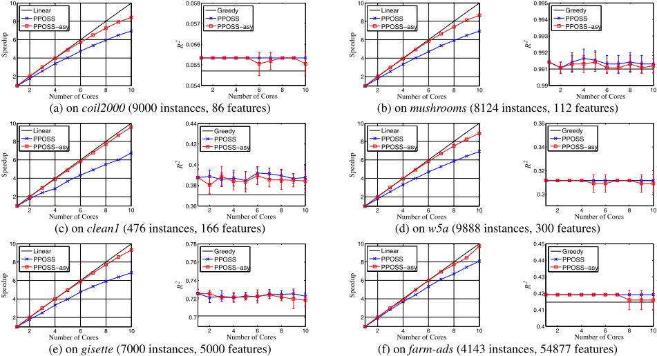
Experiments for sparse regression (Eq. (2)) are conducted on 6 data sets 1 to investigate the performance of PPOSS. We set the sparsity k = 8, and for PPOSS, we use the setting suggested by Theorem 1: T = b2ek2n◁Nc. We test the number of cores N from 1 to 10. All of the experiments are coded in Java and run on an identical configuration: a server with 4 Intel(R) Xeon(R) CPU E5-2640 v2 (8 real cores each, 20M Cache, 2.00GHz, hyper-threading) and 32GB of RAM. The kernel is Linux 2.6.18-194.el5.

We compare the speedup as well as the solution quality measured by R2 values with different number of cores N. The solution quality is also compared with that of the greedy algorithm (forward regression), which is the previous algorithm with the best known guarantee [Das and Kempe, 2011].

For PPOSS with each N value on each data set, we repeat 10 runs independently and report the average speedup and R2 values. The results are plotted in Figure 1. From the left plots in the subfigure of each data set, we can observe that PPOSS (blue line) achieves speedup around 7 when the number of cores is 10. From the right plots in each subfigure, we can see that the R2 values of PPOSS with different number of cores are stable, and better than that of the greedy algorithm except that they are the same on w5a data set. Note that on some data sets (e.g., coil2000), the standard deviation of the R2 value by PPOSS is 0, which is because PPOSS always converges to the same good solutions in 10 runs.

1 The data sets are from http://archive.ics.uci.edu/ml/ and http: //www.csie.ntu.edu.tw/⇠cjlin/libsvmtools/datasets/.

We also test the performance of PPOSS-asy, as the red lines shown in Figure 1. In the run of PPOSS-asy, all the cores share an iteration counter, and terminate until the counter reaches b2ek2nc (i.e., the number of iterations of POSS). As expected, PPOSS-asy achieves better speedup than PPOSS, because the extra cost of each iteration in the synchronous setting is avoided. Meanwhile, the R2 values obtained by PPOSS-asy are slightly worse than that of PPOSS because of the miss-synchronization.

5 Conclusion

In this paper, we propose the parallel Pareto optimization method for subset selection (PPOSS). Theoretically, we prove that for a large subclass of subset selection, PPOSS has good properties for parallelization while preserving the approximation quality: when the number of processors is limited, almost linear speedups can be achieved; with increasing number of processors, the running time can be further reduced, eventually to a constant. Note that parallel greedy methods cannot enjoy many processors, since the number of greedy steps cannot be parallelizable. This implies that, given sufficient processors, PPOSS can be both faster and more accurate than parallel greedy methods. Empirical results verify our theoretical analysis, and also show that the asynchronous PPOSS can further improve the speedup with little loss of performance.