
Bridging LSTM Architecture and the Neural Dynamics during Reading
Proceedings of the Twenty-Fifth International Joint Conference on Artificial Intelligence. Pages 1953-1958.
Abstract
Recently, the long short-term memory neural network (LSTM) has attracted wide interest due to its success in many tasks. LSTM architecture consists of a memory cell and three gates, which looks similar to the neuronal networks in the brain. However, there still lacks the evidence of the cognitive plausibility of LSTM architecture as well as its working mechanism.In this paper, we study the cognitive plausibility of LSTM by aligning its internal architecture with the brain activity observed via fMRI when the subjects read a story. Experiment results show that the artificial memory vector in LSTM can accurately predict the observed sequential brain activities, indicating the correlation between LSTM architecture and the cognitive process of story reading.
- [Bengio et al., 2003] Yoshua Bengio, Réjean Ducharme, Pascal Vincent, and Christian Janvin. A neural probabilis- tic language model. The Journal of Machine Learning Re- search, 3:1137-1155, 2003.
- [Bengio, 2009] Yoshua Bengio. Learning deep architectures for ai. Foundations and trends R in Machine Learning, 2(1):1-127, 2009.
- [Collobert and Weston, 2008] Ronan Collobert and Jason Weston. A unified architecture for natural language pro- cessing: Deep neural networks with multitask learning. In Proceedings of ICML, 2008.
- [Devereux et al., 2010] Barry Devereux, Colin Kelly, and Anna Korhonen. Using fmri activation to conceptual stim- uli to evaluate methods for extracting conceptual represen- tations from corpora. In Proceedings of the NAACL HLT Workshop on Computational Neurolinguistics, 2010.
- [Elman, 1990] Jeffrey L Elman. Finding structure in time. Cognitive science, 14(2):179-211, 1990.
- [Gabrieli et al., 1998] John DE Gabrieli, Russell A Poldrack, and John E Desmond. The role of left prefrontal cor- tex in language and memory. Proceedings of the national Academy of Sciences, 95(3):906-913, 1998.
- [Gers et al., 2000] Felix A Gers, Jürgen Schmidhuber, and Fred Cummins. Learning to forget: Continual prediction with lstm. Neural computation, 12(10):2451-2471, 2000.
- [Graves, 2013] Alex Graves. Generating sequences with re- current neural networks. arXiv preprint arXiv:1308.0850, 2013.
- [Hinton and Salakhutdinov, 2006] Geoffrey E Hinton and Ruslan R Salakhutdinov. Reducing the dimensionality of data with neural networks. Science, 313(5786):504-507, 2006.
- [Hochreiter and Schmidhuber, 1997] Sepp Hochreiter and Jürgen Schmidhuber. Long short-term memory. Neural computation, 9(8):1735-1780, 1997.
- [Karpathy et al., 2015] Andrej Karpathy, Justin Johnson, and Fei-Fei Li. Visualizing and understanding recurrent networks. arXiv preprint arXiv:1506.02078, 2015.
- [McCandliss et al., 2003] Bruce D McCandliss, Laurent Co- hen, and Stanislas Dehaene. The visual word form area: expertise for reading in the fusiform gyrus. Trends in cog- nitive sciences, 7(7):293-299, 2003.
- [Mechelli et al., 2000] Andrea Mechelli, Glyn W Humphreys, Kate Mayall, Andrew Olson, and Cathy J Price. Differential effects of word length and visual con- trast in the fusiform and lingual gyri during. Proceedings of the Royal Society of London B: Biological Sciences, 267(1455):1909-1913, 2000.
- [Mikolov et al., 2010] Tomas Mikolov, Martin Karafiát, Lukas Burget, Jan Cernockỳ, and Sanjeev Khudanpur. Re- current neural network based language model. In INTER- SPEECH, pages 1045-1048, 2010.
- [Mitchell et al., 2008] Tom M Mitchell, Svetlana V Shinkareva, Andrew Carlson, Kai-Min Chang, Vicente L Malave, Robert A Mason, and Marcel Adam Just. Pre- dicting human brain activity associated with the meanings of nouns. Science, 320(5880):1191-1195, 2008.
- [Murphy et al., 2012] Brian Murphy, Partha Talukdar, and Tom Mitchell. Selecting corpus-semantic models for neu- rolinguistic decoding. Introduction to SEM, 2012.
- [O'Reilly and Frank, 2006] Randall O'Reilly and Michael Frank. Making working memory work: a computational model of learning in the prefrontal cortex and basal gan- glia. Neural computation, 18(2):283-328, 2006.
- [Pereira et al., 2011] Francisco Pereira, Greg Detre, and Matthew Botvinick. Generating text from functional brain images. Frontiers in human neuroscience, 5, 2011.
- [Pereira et al., 2013] Francisco Pereira, Matthew Botvinick, and Greg Detre. Using wikipedia to learn semantic fea- ture representations of concrete concepts in neuroimaging experiments. Artificial intelligence, 194:240-252, 2013.
- [Price, 2000] Cathy J Price. The anatomy of language: contributions from functional neuroimaging. Journal of anatomy, 197(03):335-359, 2000.
- Rowling, 1997
- Joanne K Rowling. Harry Potter and the Philosopher Stone. 1997.
- [Schmidhuber, 2015] Jürgen Schmidhuber. Deep learning in neural networks: An overview. Neural Networks, 61:85- 117, 2015.
- [Schwartz et al., 2013] Yannick Schwartz, Bertrand Thirion, and Gaël Varoquaux. Mapping cognitive ontologies to and from the brain. In NIPS (Neural Information Processing Systems), 2013.
- [Turian et al., 2010] Joseph Turian, Lev Ratinov, and Yoshua Bengio. Word representations: a simple and general method for semi-supervised learning. In Proceedings of ACL, 2010.
- [Wehbe et al., 2014a] Leila Wehbe, Brian Murphy, Partha Talukdar, Alona Fyshe, Aaditya Ramdas, and Tom Mitchell. Simultaneously uncovering the patterns of brain regions involved in different story reading subprocesses. PloS one, 9(11):e112575, 2014.
- [Wehbe et al., 2014b] Leila Wehbe, Ashish Vaswani, Kevin Knight, and Tom Mitchell. Aligning context-based statisti- cal models of language with brain activity during reading. In Proceedings of EMNLP, 2014.
- [Yamins et al., 2014] Daniel LK Yamins, Ha Hong, Charles F Cadieu, Ethan A Solomon, Darren Seibert, and James J DiCarlo. Performance-optimized hierarchical models predict neural responses in higher visual cor- tex. Proceedings of the National Academy of Sciences, 111(23):8619-8624, 2014.
References were extracted automatically from the PDF and may contain errors.
Full text extracted automatically from the PDF; figures, tables and equations may differ. The PDF is the version of record.
1 Introduction
In recent years, biologically-inspired artificial neural networks have become a focused topic in the field of computer science [Hinton and Salakhutdinov, 2006; Bengio, 2009; Schmidhuber, 2015]. Among the various network architectures, long short-term memory neural network (LSTM) [Hochreiter and Schmidhuber, 1997] has attracted recent interest and gives state-of-the-art results in many tasks, such as time series prediction, adaptive robotics and control, connected handwriting recognition, image classification, speech recognition, machine translation, and other sequence learning problems [Schmidhuber, 2015]. LSTM is an extension of the simple recurrent neural network (RNN). It employs three gate vectors to filter information and a memory vector to store the history information. This mechanism can help encode longterm information better than simple RNN. Despite the biological inspiration of the architecture desgin of LSTM [O'Reilly and Frank, 2006] and some efforts in understanding LSTM memory cell [Karpathy et al., 2015], there still lacks the evidence of the cognitive plausibility of LSTM architecture as well as its working mechanism.
In this paper, we relate LSTM struture with the brain activities during the process of reading a story. In parallel with the fMRI experiment [Wehbe et al., 2014a], we train a LSTM neural network and use it to generate the sequential representation of the same story. By looking for the potential alignment between the representations produced by LSTM and the neural activities recorded by fMRI at the same time, we are able to explore the cognitive plausibility of LSTM architecture per se.
⇤Corresponding author.
Although some previous works [Mitchell et al., 2008; Pereira et al., 2011; 2013; Schwartz et al., 2013; Devereux et al., 2010; Murphy et al., 2012] have tried to use computational models to decode the human brain activity associated with the meaning of words, most of them focused on the isolate words. Recently, [Wehbe et al., 2014b] studied the alignment between the latent vectors used by neural networks and brain activity observed via Magnetoencephalography (MEG) when subjects read a story. Their work just focused on the alignment between the word-by-word vectors produced by the neural networks and the word-by-word neural activity recorded by MEG.
Our main contributions can be summarized as follows. First, we show that it might be possible to use brain data to understand, interpret, and illustrate what is being encoded in the LSTM architecture, by drawing parallels between the model components and the brain processes; Second, we perform an empirical study on the gating mechanisms and demonstrate the superior power of the gates except the forget gates.
2 Long Short-TermMemory Neural Network
A recurrent neural network (RNN) [Elman, 1990] is able to process a sequence of arbitrary length by recursively applying a transition function to its internal hidden state vector ht of the input sequence. The activation of the hidden state ht at time-step t is computed as a function f of the current input symbol xt and the previous hidden state ht-1
In a classic recurrent neural network, the gradient may blow up or decay exponentially over the time. Therefore, LSTM was proposed in [Hochreiter and Schmidhuber, 1997] as a solution to the vanishing gradient problem. The basic unit of LSTM consists of three gates and a memory cell, which is designed in analogy to the psychological foundation of the human memory. A number of minor modifications to the standard LSTM unit have been made. While there are numerous LSTM variants, here we describe the implementation used by [Graves, 2013].

LSTM unit has a memory cell and three gates: input gate, output gate and forget gate. Intuitively, at time step t, the input gate it controls howmuch each unit is updated, the output gate ot controls the exposure of the internal memory state, and the forget gate ft controls the amount of which each unit of the memory cell is erased. The memory cell ct keeps the useful history information which will be used for the next process.
Mathematically, the states of LSTM are updated as follows:
where xt is the input vector at the current time step, σ denotes the logistic sigmoid function and ⊙ denotes elementwise multiplication. Note that Wci, Wcf and Wco are diagonal matrices.
When we use LSTM to model the linguistic input, such as sentences and documents, the first step is to represent the symbolic data into distributed vectors, also called embeddings [Bengio et al., 2003; Collobert and Weston, 2008]. Formally, we use a lookup table to map each word as a realvalued vector. All the unseen words are regarded by a special symbol and further mapped to the same vector.
3 Methodology
Due to the complexity of LSTM, it is not always clear how to assess and compare its performances as they might be useful for one task and not the other. It is also not easy to interpret its dense distributed representations.
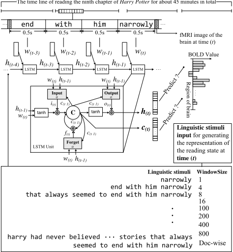
In order to explore the correlation between the LSTM architecture and human cognitive process, we employ the paradigm of mapping the artificial representation of the linguistic stimuli with the real observed neural activity, as is explained in Figure 1. One one hand, stimulated by a series of linguistic input, the neural response can be measured by the brain imaging techniques (e.g. EEG, fMRI, etc.). On the other hand, given the same series of the linguistic stimuli as the input information, an artificial model (e.g. recurrent neural network) also generates an abstract, continuous vector representation in correspondence with the real-time brain state. What would be attractive to us is whether there exists any linear mapping relationship between the model-based representation and the brain activity. This would guide us to a new direction of depicting the mechanism of model, specifically LSTM architecture in this paper. Figure 2 illustrates our experimental design.
In this section, we first briefly introduce the brain imaging data, and then we describe our experiment design.
3.1 Brain Imaging Data
The brain imaging data is originally acquired in [Wehbe et al., 2014a], which recorded the brain activities of 8 subjects when they read the ninth chapter from the famous novel, Harry Porter and the Philosopher's Stone [Rowling, 1997]. The chapter had been segmented to words so that they can be presented to the subject at the center of the screen one by one, staying for 0.5 seconds each. Since the chapter is quite long and complicated, the whole chapter was divided into four sections. Subjects had short breaks between the presentation of the different sections. Each section started with a fixation period of about 20 seconds, during which the subjects stared at a cross in the middle of the screen. The total length of the four sections was about 45 minutes. About 5180 words were presented to each subject in the story reading task.
The brain activity data is collected by the functional Magnetic Resonance Imaging (fMRI), a popular brain imaging technique used in the cognitive neuroscience research. As fMRI displays poor temporal resolution, the brain activity is acquired every 2 seconds, namely every 4 words. Details of the data acquisition can be referred to [Wehbe et al., 2014a]. Of course, there are two potential limitations with fMRI. One is the low temporal resolution, compared with EEG. The other is that fMRI BOLD (Blood Oxygenation Level Dependent) signal is an indirect measurement of the neural activities. However, its high spatial resolution and non-invasive characteristic have made it a successful tool in cognitive neuroscience, especially for human subjects. Thus, we think that it is appropriate to measure the neural dynamics with fMRI, since it has been widely accepted by the academic community.
In Figure 2, we summarize the basic information about the experiment setting of the story reading task. Taking one time step t of the whole story time line as an example, the previous 4 words 'end' (w(t-3)), 'with' (w(t-2)), 'him' (w(t-1)), 'narrowly' (w(t)) appeared on the screen one by one. The BOLD signal was recorded by the brain imaging machine after the presentation of these 4 words. Similar arrangements are carried over the other part of the reading process.
We preprocess the fMRI data before training the model to remove noise from the raw data as much as possible. We compute the default brain activity ¯ y by selecting the fMRI recording of the default state and averaging these fMRI data. Then we subtract other observed brain activity with the default brain activity ¯ y. The new fMRI data of each time step are used in the experiments.
3.2 Alignment
LSTM has two key hidden vector representations to keep the history information and be used in the next time step: (1) a memory vector ct that summarizes the history of the previous words; and (2) the hidden state vector ht that is used to predict the probability of the incoming word.
Under the paradigm of the brain-LSTM mapping experiment, the brain activity at the t-th time step of the story reading process can be viewed as a vector y(t) in the continuous high-dimensional space. Each dimension of y(t) reflects the measured value of the BOLD signal of a certain tiny area (about 3⇥3⇥3mm3 ) in the brain, which is also called voxel (VOlumeric piXEL). Mathematically, at the t-th time step, we use vector a(t) to represent the activations of internal neurons in LSTM. In this paper, a(t) may be memory vector ct and hidden state vector ht.
To align the activation a(t) of LSTM and brain activity y(t) at the same time step t, we define a function to predict the brain activity ˆ y(t) from a(t).
In this paper, we use linear function
where M is the mapping matrix between a(t) and y(t), which is learnt by the least square error.
The matrix M ⇤ is analytically solved as:
where A = [a(1)↪ · · · ↪ a(T)] and Y = [y(1)↪ · · · ↪ y(T)].
Here, we do not train a LSTM neural network to directly predict the brain activities. The reasons lie in two points.
First, the dimension of the fMRI signal varies among different subjects. Therefore, it is not convenient to design a universal neural network architecture for generating outputs of different dimensions.
Second, the goal of this research is not to improve the performance of predicting fMRI signal with LSTM neural network. We just wish to explore the characteristic of the artificial memory vector and the hidden state in the LSTM architecture, as the work on correlating the performance-optimized deep neural network models with the neural activities in the visual cortex [Yamins et al., 2014]. Therefore, we try to avoid any possible supervision from the fMRI data when training LSTM language model.
3.3 EvaluationMetric
Regarding the evaluation metric, we evaluate the model by computing the average cosine distance between the predicted functional brain image and the true observed brain activity at a certain time step of the story reading process. For each activations a(t) of LSTM at the time step t in the test cases, we compute the predicted brain activity ˆ y(t). Then we calculate the cosine distance between ˆ y(t) and y(t). Since the cosine distance lies between -1 and 1, we normalise the cosine distance into [0,1] and use it as the accuracy of each test case. We train the linear map model over about 95% of the brain imaging data and test the model over the remaining 5%. We apply 20-folds cross-validation in order to get the average performance of the model.
4 Experiment
In our experiments, the dimensionality of word embeddings is set to 50, the hidden state size is also set to 50, and the initial learning rate is set to 0.1. The other parameters are initialized by randomly sampling from uniform distribution in [-0.1, 0.1], based on the experience with recurrent neural network.
LSTM is trained according to the procedure of the neural language model [Mikolov et al., 2010], which predicts the incoming word given the history context. Since only one chapter of Harry Porter and the Philosopher's Stone is involved in the original story reading experiment, the remaining chapters of the book is used as the training data.
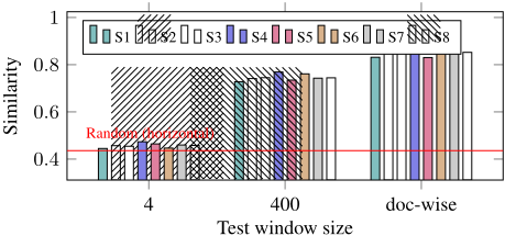
Our results report the averaged accuracies over 8 subject under the same experimental conditions. To show the feasibility of this averaging, we show the mean accuracy of LSTM
memory vector with three different experimental settings over eight subjects in Figure 1. We can see that there is not much between-subject variance. Therefore, each data point in Figure 4 is computed by averaging the accuracy of 160 test cases (8 subjects with 20 test folds each).
4.1 Effect of the Long-TermMemory
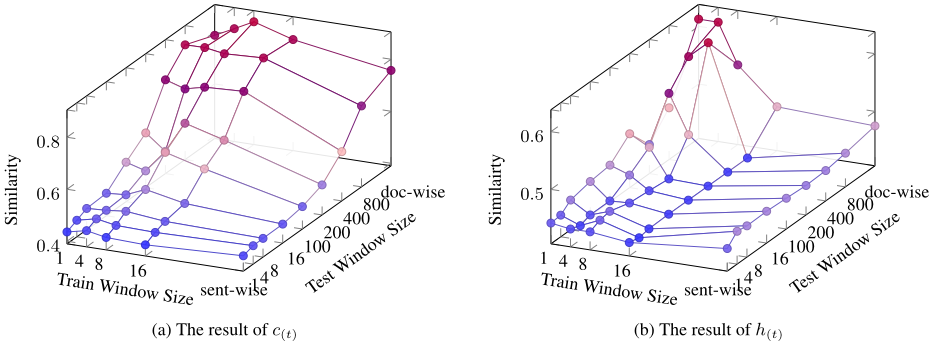
LSTM does not explicitly differentiate short-term memory with long-term memory, from a general view of its unit architecture. Therefore, in order to clearly explore how LSTM unit learns to encode the long-term and short-term information and the interaction between the two types of working memory, we deliberately cut the text data with different window size, both for the training corpus and the test stimuli. We set window size as 1, 4, 8, 16 and sentence-length for training data and 1, 4, 8, 16, 100, 200, 400, 800, document-length for test data, as is visualized in Figure 3. When training LSTM neural network and generating the vector representation a(t) for every time step t, we choose the data of the different window size for LSTM neural network.
The experiment results are presented in Figure 4, which suggests that the memory vector of LSTM neural language model generally performs significantly better than the hidden state vector of the neural network in the brain mapping task, given the same hyper-parameter configuration. Besides, the accuracy of the predicted brain image by LSTM memory vector reach about 86% at the best performance, while the highest accuracy of the predicted brain image by LSTM hidden state vector only reach about 61%. This supports the cognitive plausibility of the LSTM memory cell architecture.
Regarding the influence of the window size of the training data and the window size of the test data on the model performance, the accuracy increases with large test window size in general. As far as the hidden state vector is concerned, the accuracy also increases with small window size of the training data and the large window size of the test data.
However, we are surprised to find that the memory vector of LSTM architecture achieves the best performance when LSTM model is trained with the text data of exactly the 8word window size and generate brain activity representation with the word sequence input of the document-wise test window size, as is shown in Figure 4. The accuracy sharply decreases when the model generates the representation and predicts fMRI signals only from the previous 4 or 8 words with a limited, small test window size. The accuracy of the memory vector is very low when test window size is small, no matter we decrease or increase the window size of the training data. This indicates that the long-termmemory plays an important role in constructing the artificial memory.
4.2 Effect of the Internal Factor: the Gating Mechanisms
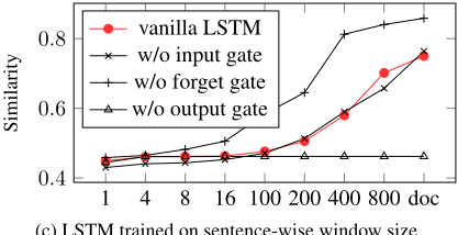
In order to take a further look at the role of each gate in the general LSTM architecture, we "remove" the input gates, the forget gates and the output gates respectively by setting their vector as a permanent all-one vector respectively. Then we train the new models with the data of the different window size. The results are presented in Figure 5. It is obvious that dropping gates brings a fatal influence to the performance on the brain image prediction task. While it may have negative impact to drop input and output gates, the performances seem to been even improved when dropping the forget gates.
Looking at the brief history of LSTM architecture, we find that the original model in [Hochreiter and Schmidhuber, 1997] only has the input gate and the output gate. [Gers et al., 2000] added a forget gate to each LSTM unit, suggesting that it will help improve the model in dealing with continual input stream. It might be the case that story reading, in our experiment, is not a tough prediction task since the size of the input stream is limited to only a part of one novel chapter. In addition, reading should involve the processing of documentwise information, which means setting forget gates to all-one vector should not pose much negative influence to the ability of the model.
It is worth noticing that the performance falls down sharply Similarity Similarity
0▷8
0▷6
0▷4
vanilla LSTM
w/o input gate
w/o forget gate
w/o output gate
1 4 8 16 100 200 400 800 doc
(a) LSTM trained on 8-word window size
vanilla LSTM
w/o input gate
w/o forget gate
w/o output gate
1 4 8 16 100 200 400 800 doc
(c) LSTM trained on sentence-wise window size
Figure 5: Comparative analysis of LSTM model with/without a certain gate. The x-axis of each sub-figure represents the window size of the test data.
when the output gates is removed. From a technical perspective, this is probably because that the output gate is close to the hidden state, which means that the output gate receives the back-propagating gradient earlier than the other two gates. The error can not be correctly updated. Therefore, removing the output gate will certainly interfere with the normal back propagation process, leading the model training process towards a wrong direction.
4.3 Comparison to Other Models
We compare LSTM model with the vanilla RNN and other heuristic models.
Vanilla RNN hidden We train a vanilla RNN language model and generate a series of representation of the story with the hidden state vector. The experiment configuration of the training and testing data are the same with that of the best LSTMmodel.
BoW (tf-idf) For time step t , we transform the text that the subject has read into a tf-idf (term frequency-inverse document frequency) representation.
0▷8
0▷6
0▷4
AveEmbedding We average the word embedding of all the words that have been read at a certain time step t to generate a representation for the brain state. We use the public Turian word embedding dataset [Turian et al., 2010].
Applying the same evaluation metric, we found that the AveEmbed heuristic model performs well, achieving a similarity of 0.81. LSTM memory vector is significantly better than the heuristic method. RNN hidden vectors, however, give out poor performance. A key reason is that RNN only captures short-term information and therefore fails in modelling reading process, which involves strong integration of the long-term information.
| Model | Cosine Dist. | Similarity |
|---|---|---|
| Random | -0.128 | 0.436 |
| BoW(tf-idf) | 0.184 | 0.592 |
| AveEmbedding | 0.634 | 0.817 |
| RNN hidden | 0.016 | 0.508 |
| LSTM hidden | 0.224 | 0.612 |
| LSTM memory | 0.724 | 0.862 |
5 Discussion
We can summary the observations from the experiment results as follows.
- ÷ LSTM has the ability to encode the semantics of a story by the memory vector, in which the stored information can be used to predict the brain activity with 86% similairty. Compared to the simple RNN, the overall architecture of LSTM should be more cognitively plausible.
- ÷ The gating mechanisms are effective for LSTM to filter the valuable information except the forget gates, which is also consistent with the adaptive gating mechanism of working memory system [O'Reilly and Frank, 2006].
- ÷ The long-term memory can be well kept by LSTM. When we deliberately cut the source of long-term memory (by using small context window size), the prediction accuracy decreases greatly.
5.1 Visualization Analysis
In addition to the quantitative analysis above, we visualize part of the brain state dynamics of subject 1 in Figure 6, including the true signal sequence at 80 randomly-selected voxels and two signal sequences reconstructed by LSTM memory vector and LSTM hidden state vector. The x-axis of each sub-figure represents the time steps of the reading process (the fixation periods between every two runs are removed). The colour indicates the activation level of a certain brain region at a certain time step.
We found that the brain dynamics reconstructed by the memory vector of LSTM is more like a smoothed version of the real brain activity. The brain dynamics reconstructed by the hidden state vector of LSTM are largely deviated from the real brain activity, although LSTM hidden state reconstructs a few features of the real brain signals.

5.2 Connection with Cognitive Neuroscience
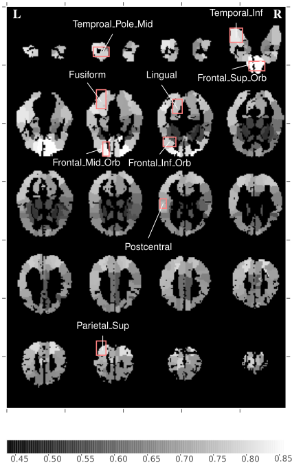
To explore whether the predictability of the neural activity varies among different brain regions for LSTM memory vector, we compute the correlation of the predicted and the real brain activities by measuring the Pearson correlation coefficient for each voxel within each subject. Then we compute the averaged correlation for a specific anatomical region defined by AAL (Automated Anatomical Labeling) atlas and visualize the correlation strength for subject 1 in Figure 7.
We notice some interesting phenomena that might reflect the association of the LSTM memory vector with the predictability of brain regions involved in language processing and semantic working memory.
[Gabrieli et al., 1998] indicates that prefrontal cortex is associated with semantic working memory. [Price, 2000] summarizes that frontal superior gyrus is associated with the processing of word meaning and that temporal pole area is associated with sentence reading. Our analysis also reflects a strong correlation between the reconstructed brain activity from LSTM memory vector and the observed brain activity of the prefrontal cortex and temporal cortex, especially the inferior and anterior part of the gyrus.
We also found that the reconstructed brain activity of Lingual gyrus and Fusiform (Visual Word Form Area ) are highly correlated with the real observed activities. Previous neuroscience research [Mechelli et al., 2000; McCandliss et al., 2003] has reported that these brain regions play an important role in word recognition. Similar patterns have also been found for other subjects.
6 Conclusion
In this paper, we explore LSTM architecture with the sequential brain signal of story reading. Experiment results suggest a correlation between the LSTM memory cell and the cognitive process of story reading. In the future work, we will continue to investigate the effectiveness of different LSTM variants by relating the representation generated by the models with neural dynamics. We would also try to design a more reasonable artificial memory architecture for a better approximation to the working memory system and language cognition. Besides, we will investigate some non-linear mapping function between the artificial and brain memories.
Acknowledgments
We would like to thank the anonymous reviewers for their valuable comments. This work was partially funded by National Natural Science Foundation of China (No. 61532011, 61473092, and 61472088), the National High Technology Research and Development Program of China (No. 2015AA015408).
@inproceedings{ijcai2016p279,
  title     = {Bridging LSTM Architecture and the Neural Dynamics during Reading},
  author    = {Qian, Peng and Qiu, Xipeng and Huang, Xuanjing},
  booktitle = {Proceedings of the Twenty-Fifth International Joint Conference on
               Artificial Intelligence, {IJCAI-16}},
  publisher = {AAAI Press / International Joint Conferences on Artificial Intelligence},
  editor    = {Subbarao Kambhampati},
  pages     = {1953--1958},
  year      = {2016},
  month     = {7},
  url       = {https://ijcai.org/proceedings/2016/279},
}
TY - CPAPER TI - Bridging LSTM Architecture and the Neural Dynamics during Reading AU - Qian, Peng AU - Qiu, Xipeng AU - Huang, Xuanjing T2 - Proceedings of the Twenty-Fifth International Joint Conference on Artificial Intelligence, IJCAI-16 PB - AAAI Press / International Joint Conferences on Artificial Intelligence PY - 2016 SP - 1953 EP - 1958 UR - https://ijcai.org/proceedings/2016/279 ER -Copied
Machine-readable versions of this paper, for tools and AI agents:





