
Distance Based Modeling of Interactions in Structured Regression
Proceedings of the Twenty-Fifth International Joint Conference on Artificial Intelligence. Pages 2032-2037.
Abstract
Graphical models, as applied to multi-target prediction problems, commonly utilize interaction terms to impose structure among the output variables. Often, such structure is based on the assumption that related outputs need to be similar and interaction terms that force them to be closer are adopted. Here we relax that assumption and propose a feature that is based on distance and can adapt to ensure that variables have smaller or larger difference in values. We utilized a Gaussian Conditional Random Field model, where we have extended its originally proposed interaction potential to include a distance term. The extended model is compared to the baseline in various structured regression setups. An increase in predictive accuracy was observed on both synthetic examples and real-world applications, including challenging tasks from climate and healthcare domains.
- [Bakir et al., 2007] Gökhan Bakir, Thomas Hofmann, Bern- hard Schölkopf, Alexander J Smola, Ben Taskar, and S.V.N. Vishwanathan. Predicting Structured Data. MIT Press, 2007.
- [Dunlop et al., 2008] Mary J Dunlop, Robert Sidney Cox, Joseph H Levine, Richard M Murray, and Michael B Elowitz. Regulatory activity revealed by dynamic cor- relations in gene expression noise. Nature genetics, 40(12):1493-1498, 2008.
- [Friedman et al., 2008] Jerome Friedman, Trevor Hastie, and Robert Tibshirani. Sparse inverse covariance estima- tion with the graphical lasso. Biostatistics, 9(3):432-441, 2008.
- [Gligorijevic et al., 2016] Djordje Gligorijevic, Jelena Sto- janovic, and Zoran Obradovic. Uncertainty Propagation in Long-term Structured Regression on Evolving Networks. In Thirtieth AAAI Conference on Artificial Intelligence (AAAI-16), 2016.
- [Kalnay et al., 1996] Eugenia Kalnay, Masao Kanamitsu, Robert Kistler, William Collins, Dennis Deaven, Lev Gandin, Mark Iredell, Suranjana Saha, Glenn White, John Woollen, et al. The NCEP/NCAR 40-year reanalysis project. Bulletin of the American meteorological Society, 77(3):437-471, 1996.
- [Kim and Xing, 2009] Seyoung Kim and Eric P Xing. Sta- tistical estimation of correlated genome associations to a quantitative trait network. PLoS Genet, 5(8):e1000587, 2009.
- [Kumar and Hebert, 2004] Sanjiv Kumar and Martial Hebert. Discriminative Fields for Modeling Spatial Dependencies in Natural Images. In Advances in Neural Information Processing Systems, pages 1531-1538, 2004.
- [Lafferty et al., 2001] John Lafferty, Andrew McCallum, and Fernando CN Pereira. Conditional random fields: Probabilistic models for segmenting and labeling sequence data. ICML, pages 282-289, 2001.
- [Menne et al., 2009] Matthew J Menne, Claude N Williams Jr, and Russell S Vose. The US Historical Climatology Network monthly temperature data, version 2. Bulletin of the American Meteorological Society, 90(7):993, 2009.
- [Ng and Jordan, 2002] Andrew Ng and Michael Jordan. On discriminative vs. generative classifiers: A comparison of logistic regression and naive bayes. Advances in NIPS, 14:841-848, 2002.
- [Peng and McCallum, 2006] Fuchun Peng and Andrew Mc- Callum. Information extraction from research papers us- ing conditional random fields. Information processing & management, 42(4):963-979, 2006.
- [Radosavljevic et al., 2010] Vladan Radosavljevic, Slobo- dan Vucetic, and Zoran Obradovic. Continuous Condi- tional Random Fields for Regression in Remote Sensing. In Proceedings of the 19th European Conference on Arti- ficial Intelligence (ECAI 2010) Lisbon, Portugal, 2010.
- [Radosavljevic et al., 2013] Vladan Radosavljevic, Kosta Ristovski, and Zoran Obradovic. Gaussian Conditional Random Fields for Modeling Patients Response to Acute Inflammation Treatment. In ICML 2013 workshop on Ma- chine Learning for System Identification, 2013.
- [Radosavljevic et al., 2014] Vladan Radosavljevic, Slobo- dan Vucetic, and Zoran Obradovic. Neural Gaussian Con- ditional Random Fields. In Machine Learning and Knowl- edge Discovery in Databases, pages 614-629. Springer, 2014.
- [Sato and Sakakibara, 2005] Kengo Sato and Yasubumi Sakakibara. RNA secondary structural alignment with conditional random fields. Bioinformatics, 21(suppl 2):ii237-ii242, 2005.
- SID), 2003 2011] HCUP State Inpatient Databases (SID). Healthcare Cost and Utilization Project (HCUP). www. hcup-us.ahrq.gov/sidoverview.jsp, 2003-2011. Agency for Healthcare Research and Quality, Rockville, MD. Link
- [Sohn and Kim, 2012] Kyung-Ah Sohn and Seyoung Kim. Joint estimation of structured sparsity and output struc- ture in multiple-output regression via inverse-covariance regularization. In International Conference on Artificial Intelligence and Statistics, pages 1081-1089, 2012.
- [Stojanovic et al., 2015] Jelena Stojanovic, Milos Jovanovic, Djordje Gligorijevic, and Zoran Obradovic. Semi- supervised learning for structured regression on partially observed attributed graphs. In Proceedings of the 2015 SIAM International Conference on Data Mining (SDM 2015) Vancouver, Canada. SIAM, 2015.
- [Sutton and McCallum, 2006] Charles Sutton and Andrew McCallum. An introduction to conditional random fields for relational learning. Introduction to statistical relational learning, pages 93-128, 2006.
- [Tappen et al., 2007] Marshall F Tappen, Ce Liu, Edward H Adelson, and William T Freeman. Learning gaussian conditional random fields for low-level vision. In IEEE Conference on Computer Vision and Pattern Recognition, (CVPR'07), pages 1-8. IEEE, 2007.
- [Wytock and Kolter, 2013] Matt Wytock and Zico Kolter. Sparse Gaussian conditional random fields: Algorithms, theory, and application to energy forecasting. In Pro- ceedings of the 30th International Conference on Machine Learning (ICML-13), pages 1265-1273, 2013.
- [Ye and Liu, 2012] Jieping Ye and Jun Liu. Sparse methods for biomedical data. ACM SIGKDD Explorations Newslet- ter, 14(1):4-15, 2012.
References were extracted automatically from the PDF and may contain errors.
Full text extracted automatically from the PDF; figures, tables and equations may differ. The PDF is the version of record.
1 Introduction
Structured prediction is a technique of simultaneously predicting a set of related response variables given a set of explanatory variables [Bakir et al., 2007]. Many of the challenges in structured prediction are due to the exponential size of that multi-variable output space, requiring complex models to represent the problem, which further reflects on the feasibility and tractability of learning and inference algorithms. The resulting variables used to describe the object of interest are often interrelated, and relations between variables form a structure. That structure, although potentially complex, can usually be leveraged to make the problem feasible.
Structured regression, as opposed to structured classification, requires the set of response variables to have continuous values. A challenge in structured regression is optimization efficiency, as optimization is used at both the learning and inference stages. Common modeling approaches to structured regression are undirected Probabilistic Graphical Models named Markov Networks, or Markov Random Fields (MRF). The choice of models that express joint or conditional distributions depends on task objectives, training examples availability, and other constraints [Ng and Jordan, 2002]. Discriminative models are often preferred over generative ones as more accurate due to relaxations of independence assumptions [Sutton and McCallum, 2006]. That is why Conditional Random Fields [Lafferty et al., 2001] are extensively applied in various domains, including Computer Vision [Peng and McCallum, 2006], Natural Language Processing problems [Kumar and Hebert, 2004] and Bioinformatics [Sato and Sakakibara, 2005]. However, common choice of the feature functions' type, particularly the interaction functions, are limiting the potential of the model in certain cases. A typical assumption is that if variables are related, they should be more similar. The interaction potential is then constructed in such a way that it penalizes difference between the connected response variables, making them more similar and therefore acting as a smoother. This assumption is also present in other applications of graphical models that penalize difference in related variables, like feature selection with Graphical LASSO [Friedman et al., 2008]. However, sometimes this smoothing is an undesirable property and one proposed solution to that problem was introducing the sign term when subtracting the values of two outputs, resulting in Graphical Fused LASSO penalty [Kim and Xing, 2009]. That trick is not always adequate for use, since it introduces problems when the sign is misspecified and because of its hard discontinuity [Ye and Liu, 2012].
Here, we propose a generalization of the most commonly used interaction potential function, namely the one operating on a difference of pairs of variables. We extend it to include the difference (distance) term, which broadens the scope of its application. It is no longer acting exclusively as a smoother, but it could also make variables more different (distant), if needed. With such interaction potential, the model will try to force the difference between variables to be equal to the specified distance term. In this paper, we study the behaviour of such interaction functions on the Gaussian Conditional Random Fields (GCRF) model. In the proposed approach, inference and learning properties of original model remain preserved, and the scope of its acting is extended beyond the smoothing, resulting in increased accuracy in structured regression tasks. The original model is in fact a special case of the proposed model when distance terms are set to zeros.
Related work on GCRF models, our proposed model and the interpretation of the extension are described in Section II. Experimental results are presented in Section III, followed by conclusions presented in Section IV.
2 Model
Although representationally powerful, applications of Continuous Conditional Random Fields to modeling problems is somewhat hampered by the high computational complexity related to calculating the partition function (normalization term). Also, in general, inference on them requires expensive sampling methods. To alleviate some of those problems and make the methods more applicable, the Gaussian distribution assumption can be imposed. Recently, several formulations of CRF models named Gaussian Conditional Random Fields (GCRF) were proposed [Tappen et al., 2007; Radosavljevic et al., 2010; Sohn and Kim, 2012; Wytock and Kolter, 2013]. Approaches like [Wytock and Kolter, 2013; Sohn and Kim, 2012] utilize regularization techniques, mainly L1 norm, to impose sparseness and learn the precision matrix and its structure. Others, like [Tappen et al., 2007], have more specialized formulation tightly related to the application of interest. Radosavljevic et al. [2010] proposed a model for AOD prediction and regression in remote sensing, which relies on a known structure to constrain the learning of the predictive model, and in this work we are going to focus on this particular kind of GCRF. It utilizes a formulation of feature functions where the resulting probability has multivariate Gaussian form. This property of GCRF allows efficient inference in the form of an algebraic solution. Moreover the resulting GCRF learning (parameter fitting) problem is convex, which allows the use of reliable optimization algorithms and guarantees a high quality solution. All these characteristics make GCRF a promising tool for a broad spectrum of applications including climate [Radosavljevic et al., 2010], and health-care [Radosavljevic et al., 2013] and it has been modified in several different ways [Radosavljevic et al., 2014; Stojanovic et al., 2015; Gligorijevic et al., 2016].
2.1 Related work
One of the challenges in structured learning is finding the appropriate structure for the problem at hand.
As outlined previously, there are several approaches to structured learning with Gaussian Conditional Random Fields, corresponding to different parameter sharing and the need and ability to learn the structure itself. One approach is based on learning the covariance matrix ([Wytock and Kolter, 2013], [Sohn and Kim, 2012]) using sparsity-inducing regularization. This approach utilizes no parameter sharing, thus effectively learning the entire (but sparse) structure. Another approach is based on exploiting additional information in the form of a predefined weighted graph [Radosavljevic et al., 2010]. Usually, this kind of additional information comes from domain knowledge or underlying topology of the problem. Here we will adopt a hybrid approach, where sparsity is predefined by the presence of the edges in the graph, but the weights of edges are learned as model parameters. The motivation for this is based on the following: if learning the whole structure only from the data, sparse learning methods must be employed since otherwise too many parameters need to be determined; however, when a structure is predefined, the model largely depends on the quality of the given structure.
To present our model, we will first describe the work of [Radosavljevic et al., 2010], where a model is defined as a weighted product of association and interaction potentials:
Here, each association potential is defined as a squared difference between node response variable yi and some independently estimated value Ri obtained as an unstructured predictor. Several association potentials can be associated with each node, corresponding to different predictions of the node value. An interaction potential is defined as a weighted squared difference between the response variable at neighboring nodes in a graph, with the weight Sij being proportional to the corresponding edge in the graph. Several sets of association and interaction potentials corresponding to different unstructured predictors can be used, hence summation over k and l in (1). Weighting factors ↵ and β for the association and interaction potentials are the parameters of the model and can be learned using the maximum likelihood optimization.
This model relies on a predefined structure given in a form of an undirected weighted graph S. For some problems this graph arises naturally, e.g. when correlation patterns can be easily identified, as in spatial or temporal problems. When a graph is suitably chosen, the parameter space is greatly reduced, allowing the efficient learning. However, if the chosen graph is not appropriate for the problem, the parameter space is restricted to a subspace of the original problem that may not contain the desired solution, and underfiting may occur.
The interaction potential functions defined in (1) penalize the difference between the predictions at neighboring nodes, thus acting as a smoothing filter. The intensity of penalization is proportional to the edge weight.
Efficient inference on this model is possible since expression (1) can actually be represented as a multivariate Gaussian conditional distribution. The partition function therefore has an analytic solution, and mode is simply the mean of the multivariate Gaussian. The likelihood function is a convex function of ↵ and β parameters, and reliable and effective optimization methods can be used.
2.2 The proposed model
Commonly, the model described in (1) is viewed as a sum of weighted potentials appearing as the exponent of a base of a natural logarithm e. Here we present it from a different perspective, and focusing on the model as a multiplication of Gaussian functions. This viewpoint will make it easier to point out some important characteristics. In general, MRF (and CRF) with single and pairwise potentials on the set of n variables Y = [y1▷▷▷yn]T , can be factored as:
While MRF models both response Y and covariates X jointly, CRF models only the conditional probability of Y given X. The convenience of the conditional model is that by omitting structure between covariates, parameter space can be significantly reduced. We are interested in regression of the response variables from a set of measured explanatory variables, therefore, from now on we will discuss the CRF model.
If we adopt the Gaussian functions for activation potentials (fi) and interaction potentials (gij ) we obtain a Gaussian conditional random field. If we now rewrite activation potentials from model (1), they will have the form of a Gaussian function with parameters (R↪ σ):
where Ri(X) is the mean estimated from the data with some regression method, and which depends on the values of explanatory variables. Term σ2 i = 12 ↵-1 represents the variance as a function of a shared parameter ↵ to be learned.
Interaction potentials also have the Gaussian function form with parameters (0↪ σij):
where: ∆yij = yi - yj , the mean is zero and variance is σ2 ij = (2βSij)-1 , β is a shared parameter to be learned. Interpretation of (3) and (4) is the following:
- Gaussian function association potentials (3) force the value of each yi to be near the corresponding Ri(X), with precision parameter p↵ to be learned.
- Gaussian function interaction potentials (4) force a value of ∆yij to be close to zero, with precision proportional to pSij. Therefore, Sij can be interpreted as a similarity measure (greater values of Sij indicate smaller ∆yij). Proportionality factor pβ for interactions is learned as a model parameter.
This form of interaction function with zero mean forces related variables to be more similar. That characteristic might be desirable under the assumption that related variables should always be similar, but that doesn't necessarily need to be the case. Therefore, we extend the interaction potential model (4) by introducing an additional term Dij(X), which represents a distance measure which depends solely on X:
The new GCRF model can now be stated as:
Interpretation of model in (6), which we refer to as Distance GCRF or DGCRF, is as follows:
- Gaussian function association potentials remain the same as in original GCRF [Radosavljevic et al., 2010], with the exception that there is no parameter sharing between nodes.
- Gaussian function interaction potentials (5) now force the difference between the i-th and j-th node to be exactly Dij(X). Precision (interaction "strength") of each pair (yi↪ yj) is proportional to pβij.
One can notice that in the new formulation there is no similarity term Sij, and the reason is that now when we have separate βij for each edge (not shared parameter anymore) we no longer need prespecified Sij to weight total precision associated with each term. Now those precision parameters can be learned much more appropriately through the model.
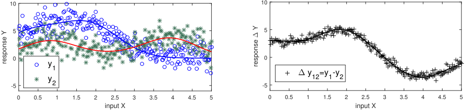
In order for the method to work well, the appropriate distance values need to be determined. We propose learning these parameters in a similar way as learning the single output variables, which is fitting Ri(X) using regression methods, except now we will regress the difference ∆yi↪j between variables yi and yj from the input X. One might ask why to fit the difference as a function of input if we have already fitted the output variables themselves. Shouldn't the difference model just be the difference between the two models? That doesn't necessarily need to be the case. We can consider an example illustrated at Figure 1 where variables have highly correlated noise. When fitting the variables, noise might prevent us from getting some of the true information and also make us pick information that comes from the noise (Figure 1 left panel). However, when fitting the difference of those two variables (Figure 1 right panel), highly correlated noise might cancel a significant part of itself and allow us to pick up more reliable information than in the case of original outputs. That is one mechanism that could justify including information about the difference of signals into the model.
2.3 Inference and learning
The newly proposed model has inherited all the convenient properties from the baseline model.
We will first examine inference. The modeled conditional probability takes the form:
If we equate the exponent of a model in (7) as a sum of weighted quadratic potentials (8) and the exponent as a multivariate Gaussian (9):
We obtain that precision matrix Q = ⌃-1 is composed of Q1 (association potential part) and Q2 (the interaction potential part):
We also get that
Therefore, b takes the following form:
Since the difference is anti-symmetric, Dij(X) = -Dji(X), it can be used to train only one direction, and then the other one is estimated just as its negation, and fed to the appropriate place in (13).
Since ⌃-1 = 2(Q1+Q2), using equations (10) to (13) we can infer the vector of most probable values for the variables of interest.
We can also notice that inference of the newly proposed model differs from the original only in the equation for b, where the original model equation is made from just the first sum in (13).
Free parameters alphas and betas are commonly learned from data (and provided independence structure) by maximizing the log-likelihood.
Here we provide derivatives of the log-likelihood for the parameters of the model. We start from the expression d log P as stated in [Radosavljevic et al., 2010]:
From which we get a particular derivative function for each parameter:
where matrices I (i) , I (i↪j) are derivatives of the precision matrix over parameters ↵i and βij respectively, and vectors V (i) , V (i↪j) are derivatives of the b vector over the same parameters.
2.4 Behaviour of the model
An analogy can be drawn between the behaviour of the originally introduced interaction potential from (4) and a rubber band. The weighting coefficient in interaction potential similarly behaves as the band's stiffness coefficient; the higher it is the less tolerant it will be to difference in their values and the higher the force it will try to reduce it with. More importantly, it may only reduce the difference, it can never make it larger, the band cannot push its ends away from itself. In some cases, estimated values of two variables actually need to be pushed apart. In the graphical models with discrete valued variables, such pairs are called "repulsive nodes". Newly introduced interaction potential eq. (5) does not force the variables to have exactly zero difference, instead, it allows the tuning of that distance parameter to some other, potentially more appropriate value. Once that distance parameter is fixed, the interaction potentials force the neighbouring values to that difference. If the values are too far apart (where estimated distance should be smaller) it will bring them closer, similarly as the original GCRF. However, if they are too close together, it will move them apart towards the desired distance. This behaviour is different than the rubber band model and it can be seen as a spring model, where springs have some nominal length which they will keep at rest. But if one tries to stretch a string or to compress it, it will resist towards its nominal condition.
2.5 Computational cost
Since the baseline model approximated the mean parameters of interaction potential with zeros, it didn't need to build the regression models for them. The newly proposed model has to do it, which results in increased effort to build the model. In the worst case of a dense structure, the number of single target models that has to be fitted is quadratic with the size of the problem. Luckily, the structure in problems of interest is often sparse and computationally manageable, as will be demonstrated in the results section. Many complex systems like biological and social processes tend to have a scale-free property characterized by a power law degree distribution, which results in a practically linear number of links in the number of nodes. In such a case, the computational complexity of fitting the unstructured models is proportional to that of the baseline models.
Regarding the increase in the number of free parameters of the model, which we have introduced by relaxing the sharing of the parameters, it also increases the computational burden. That cost is reflected in the fact that more iterations need to be performed in order for the optimization algorithm to converge in higher dimensional parameter space. However, the asymptotic computational complexity remains the same, since the main computational burden still comes from the matrix inversion.
With all that in mind, the newly proposed method does have an additional computational cost compared to the baseline, but it is applicable on every problem where the baseline can be applied, since they share the same limitations regarding the size of the problem.
3 Experimental Results
In order to characterize the improved capabilities of the extended model over the baseline model we have conducted a number of computational experiments described in the following two subsections.
3.1 Synthetic data
The GCRF model is based on an assumption that the process that generates samples has a deterministic function for the mean and the covariance that also might depend on the input space of the problem. The model assumes that there are multiple output (response) variables that are to be predicted, while the input space (the variables the joint distribution is conditioned on) may or may not be multidimensional. Mean functions of the synthetic examples are created as parametrized polynomials with (pseudo)random parameters, and correlated noise is superimposed to them in order to include the relation (structure) between those targets. As the structure pattern between the variables, we have set two prototypical examples, linear chain and regular two dimensional grid (mesh). Such structures are simple, sparse and artificially generated, yet they can provide an appropriate representation for various problems present in temporal or genomic sequence of events, and in spacial applications.
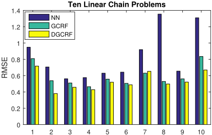
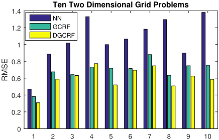
In our first type of synthetic experiments 10 examples of the linear chain connection structure of 10 variables are considered. The connection between the variables in the chain is expressed as an appropriate sparse precision matrix. Similarly, in the second type of synthetic examples, the grid structure containing 9 nodes (3 x 3), is created as ten random initializations of mean and noise patterns.
In our experiments on synthetic data we have sampled 250 instances from the previously described process for training the neural network models (NN), which were chosen as an unstructured predictor. Another 150 examples are used for the unstructured models to generate predictions on which we have trained the baseline GCRF and the Distance GCRF. Both approaches relied on unstructured predictions and were tested on another 600 test examples and prediction performance was measured as the root mean squared error (RMSE). Results presented in Table 3.1 (also shown at the Figure 2) are average performance over ten different synthetic datasets.
| Method | Linear Chain | 2DGrid |
|---|---|---|
| Unstructured-NN | 0▷830◦0▷295 | 1▷052◦0▷270 |
| Structured-GCRF | 0▷594◦0▷128 | 0▷688◦0▷127 |
| Structured-DGCRF |
Structured-DGCRF 0▷533◦0▷111 0▷598◦0▷134
Table 3.1 Predictive error RMSE of three methods on two graph types. The best performance for each type is marked in bold (p-values, 0.011 and 0.0043).
The proposed DGCRF model, with distance based interaction potential as in (5), is able to improve accuracy (statistically significant with cut off level 0.05) based on information from estimation of differences between connected outputs.
3.2 Real Applications
The proposed method is further characterized and compared to alternatives on two challenging real world applications briefly described in this section.
Sepsis Admissions Prediction in California Hospitals (SEPSIS). The monthly admission rate is predicted for sepsis in the California hospitalization dataset [(SID), 2003 2011], which contained admission information for 108 months at 231 hospitals. Data for this experiment was provided by the Health Care and Utilization Project (HCUP) and State Inpatient Databases (SID). Sepsis is a diagnosis with one of the highest mortality rates in the USA. An accurate prediction of the total number of patients diagnosed with sepsis can help optimize hospital resources and reduce associated costs. In our experiments, time series consisting of sepsis related inpatient hospital records from 231 hospitals were considered. The admission rate for the following month are predicted from the previous three months' admission rates for each hospital. At each node in a graph representing 231 hospitals in California we trained unstructured predictors using data from the initial 75 months. This is repeated 10 times by sampling 50 out of 75 months at random where remaining 25 months were used to learn the parameters of a structured model. The future 30 months were used as a test set in each of ten experiments. Hospital similarity matrix was derived from hospital statistics data in order to provide structure for our models. Similarity between hospitals is measured by Jensen-Shannon divergence on the mortality rate distributions, and only the large coefficients were kept in order to obtain a sparse graph of highly related hospitals.
Precipitation Estimation in Continental US (RAIN). The rain dataset contains precipitation records from meteorological stations across the USA and has been acquired from NOAA's National Climate Data Center (NCDC) [Menne et al., 2009]. We have considered monthly precipitation measurements over a period of 708 months in 1132 locations. In addition to precipitation, we used 6 variables acquired from the NCEP/NCAR Reanalysis 1 project [Kalnay et al., 1996]: Lagrangian tendency of air pressure (omega), precipitable water, relative humidity, temperature, zonal and meridional components of the wind, which are commonly used to predict climate parameters (data available on NOAA website: http://www.esrl.noaa.gov/psd/). We have utilized these variables to estimate the precipitation levels. Predictive models were trained by randomly selecting 250 months from the initial 400 months repeated 10 times, while structured models were learned on the remaining 150 months and performance was assessed on the future 308 months. We have generated the interaction structure by creating a spacial proximity graph based on three nearest locations, as it is expected that nearby sites will have similar climates.
In both experiments on real applications, the DGCRF model was more accurate as compared to the alternative models (Table 3.2). The unstructured model used for predictions in both of the structured approaches is Gaussian Process Regression (GPR) with Gaussian kernel, where hyperparameters were tuned on the training data by maximizing the marginal likelihood. Improvement in the accuracy of DGCRF, as compared to the baseline GCRF, in a two-sided t-test was statistically significant (p-value 2.5e-9 and 7.8e-8 on rain and sepsis datasets, respectively). The overall results suggest an advantage in using the distance based interaction potential model DGCRF over the baseline GCRF.
| Method | RAIN | SEPSIS |
|---|---|---|
| Unstructured-GPR | 1▷799◦0▷010 | 1▷272◦0▷020 |
| Structured-GCRF | 1▷790◦0▷007 | 1▷265◦0▷020 |
| Structured-DGCRF |
Structured-DGCRF 1▷767◦0▷004 1▷238◦0▷018
Table 3.2 Prediction error (RMSE) on two real world applications. The best performance is marked in bold.
4 Conclusion
In this study we have proposed modeling the interaction between the response variables in a network based on distance and have provided evidence that such an approach is more accurate than similarity based alternatives used in published methods. This is achieved by reformulating the GCRF model and extending the model to allow a nonzero mean parameter in the interaction potential. An additional degree of freedom introduced by the DGCRF model has resulted in increase in prediction accuracy over the commonly used baseline model, as demonstrated on number of synthetic and two real world datasets. Moreover, the proposed extension haven't jeopardized attractive computational properties of a closed form inference and convex learning of parameters in structured regression. Although the presented distance based interaction modeling is particularly suited to the GCRF models, it is not limited to use only in such models, and other graphical methods can be easily improved by the proposed approach as well.
Acknowledgments
This research was supported in part by DARPA grant FA9550-12-1-0406 negotiated by AFOSR, NSF BIGDATA grant 14476570 and ONR grant N00014-15-1-2729. Nationwide Inpatient Sample (NIS) Healthare Cost and Utilization Project (HCUP), Agency for Healthcare Research and Quality provided data used in this study.
@inproceedings{ijcai2016p290,
  title     = {Distance Based Modeling of Interactions in Structured Regression},
  author    = {Stojkovic, Ivan and Jelisavcic, Vladisav and Milutinovic, Veljko and Obradovic, Zoran},
  booktitle = {Proceedings of the Twenty-Fifth International Joint Conference on
               Artificial Intelligence, {IJCAI-16}},
  publisher = {AAAI Press / International Joint Conferences on Artificial Intelligence},
  editor    = {Subbarao Kambhampati},
  pages     = {2032--2037},
  year      = {2016},
  month     = {7},
  url       = {https://ijcai.org/proceedings/2016/290},
}
TY - CPAPER TI - Distance Based Modeling of Interactions in Structured Regression AU - Stojkovic, Ivan AU - Jelisavcic, Vladisav AU - Milutinovic, Veljko AU - Obradovic, Zoran T2 - Proceedings of the Twenty-Fifth International Joint Conference on Artificial Intelligence, IJCAI-16 PB - AAAI Press / International Joint Conferences on Artificial Intelligence PY - 2016 SP - 2032 EP - 2037 UR - https://ijcai.org/proceedings/2016/290 ER -Copied
Machine-readable versions of this paper, for tools and AI agents:





