
Inference Machines for Nonparametric Filter Learning
Proceedings of the Twenty-Fifth International Joint Conference on Artificial Intelligence. Pages 2074-2080.
Abstract
Data-driven approaches for learning dynamic models for Bayesian filtering often try to maximize the data likelihood given parametric forms for the transition and observation models. However, this objective is usually nonconvex in the parametrization and can only be locally optimized. Furthermore, learning algorithms typically do not provide performance guarantees on the desired Bayesian filtering task. In this work, we propose using inference machines to directly optimize the filtering performance. Our procedure is capable of learning partially-observable systems when the state space is either unknown or known in advance. To accomplish this, we adapt PREDICTIVE STATE INFERENCE MACHINES (PSIMs) by introducing the concept of hints, which incorporate prior knowledge of the state space to accompany the predictive state representation. This allows PSIM to be applied to the larger class of filtering problems which require prediction of a specific parameter or partial component of state. Our PSIM+HINTS adaptation enjoys theoretical advantages similar to the original PSIM algorithm, and we showcase its performance on a variety of robotics filtering problems.
- [Abbeel and Ng, 2005] Pieter Abbeel and Andrew Y Ng. Learning first-order markov models for control. In NIPS, pages 1-8, 2005.
- [Aguirre et al., 2005] Luis Antonio Aguirre, Bruno Otávio S Teixeira, and Leonardo Antônio B Tôrres. Using data- driven discrete-time models and the unscented kalman fil- ter to estimate unobserved variables of nonlinear systems. Physical Review E, 72(2):026226, 2005.
- [Bagnell et al., 2010] J Andrew Bagnell, Alex Grubb, Daniel Munoz, and Stephane Ross. Learning deep inference ma- chines. The Learning Workshop, 2010.
- [Boots et al., 2011] Byron Boots, Sajid M Siddiqi, and Ge- offrey J Gordon. Closing the learning-planning loop with predictive state representations. IJRR, 30(7):954-966, 2011.
- [Boots et al., 2013] Byron Boots, Arthur Gretton, and Geof- frey J. Gordon. Hilbert space embeddings of predictive state representations. In UAI-2013, 2013.
- [Boots, 2012] Byron Boots. Spectral Approaches to Learn- ing Predictive Representations. PhD thesis, Carnegie Mel- lon University, December 2012.
- [Breiman, 2001] Leo Breiman. Random forests. Machine learning, 45(1):5-32, 2001.
- [Chen et al., 2012] Yutian Chen, Max Welling, and Alex Smola. Super-samples from kernel herding. arXiv preprint arXiv:1203.3472, 2012.
- [Hamel and Mahony, 2006] Tarek Hamel and Robert Ma- hony. Attitude estimation on SO(3) based on direct inertial measurements. In ICRA, pages 2170-2175. IEEE, 2006.
- [Hefny et al., 2015] Ahmed Hefny, Carlton Downey, and Geoffrey J Gordon. Supervised learning for dynamical system learning. In NIPS, 2015.
- [Hsu et al., 2012] Daniel Hsu, Sham M Kakade, and Tong Zhang. A spectral algorithm for learning hidden markov models. Journal of Computer and System Sciences, 78(5):1460-1480, 2012.
- [Ko and Fox, 2009] Jonathan Ko and Dieter Fox. Gp- bayesfilters: Bayesian filtering using gaussian process pre- diction and observation models. Autonomous Robots, 27(1):75-90, 2009.
- [Langford et al., 2009] John Langford, Ruslan Salakhutdi- nov, and Tong Zhang. Learning nonlinear dynamic mod- els. In ICML, pages 593-600. ACM, 2009.
- [Littman et al., 2001] Michael L Littman, Richard S Sutton, and Satinder P Singh. Predictive representations of state. In NIPS, volume 14, pages 1555-1561, 2001.
- [Nishiyama et al., 2016] Yu Nishiyama, Amir Hossein Af- sharinejad, Shunsuke Naruse, Byron Boots, and Le Song. The nonparametric kernel Bayes smoother. In AISTATS, 2016.
- [Rahimi and Recht, 2007] Ali Rahimi and Benjamin Recht. Random features for large-scale kernel machines. In NIPS, pages 1177-1184, 2007.
- [Ross et al., 2011a] Stéphane Ross, Geoffrey J Gordon, and J Andrew Bagnell. A reduction of imitation learning and structured prediction to no-regret online learning. AIS- TATS, 2011.
- [Ross et al., 2011b] Stephane Ross, Daniel Munoz, Martial Hebert, and J Andrew Bagnell. Learning message-passing inference machines for structured prediction. In CVPR, 2011, pages 2737-2744. IEEE, 2011.
- [Roweis and Ghahramani, 1999] Sam Roweis and Zoubin Ghahramani. A unifying review of linear gaussian mod- els. Neural computation, 11(2):305-345, 1999.
- [Siddiqi et al., 2010] Sajid Siddiqi, Byron Boots, and Geof- frey J. Gordon. Reduced-rank hidden Markov models. In AISTATS, 2010.
- [Singh et al., 2004] Satinder Singh, Michael R. James, and Matthew R. Rudary. Predictive state representations: A new theory for modeling dynamical systems. In UAI, 2004.
- [Song et al., 2010] Le Song, Byron Boots, Sajid M Siddiqi, Geoffrey J Gordon, and Alex J Smola. Hilbert space em- beddings of hidden markov models. In ICML, pages 991- 998, 2010.
- [Sun et al., 2015] Wen Sun, Arun Venkatraman, Byron Boots, and J Andrew Bagnell. Learning to filter with predictive state inference machines. arXiv preprint arXiv:1512.08836, 2015.
- [Thrun et al., 2005] Sebastian Thrun, Wolfram Burgard, and Dieter Fox. Probabilistic robotics. MIT press, 2005.
- [Van Overschee and De Moor, 2012] Peter Van Overschee and BL De Moor. Subspace identification for linear sys- tems: Theory-Implementation-Applications. Springer Sci- ence & Business Media, 2012.
- [Venkatraman et al., 2015] Arun Venkatraman, Martial Hebert, and J Andrew Bagnell. Improving multi-step prediction of learned time series models. In AAAI, pages 3024-3030, 2015.
- [Wan and Van Der Merwe, 2000] Eric A Wan and Ronell Van Der Merwe. The unscented kalman filter for nonlinear estimation. In AAS-SPCC, pages 153-158. IEEE, 2000.
- [Wei, 1994] William Wu-Shyong Wei. Time series analysis. Addison-Wesley publ, 1994.
- [Zinkevich, 2003] Martin Zinkevich. Online Convex Pro- gramming and Generalized Infinitesimal Gradient Ascent. In ICML, pages 421-422, 2003.
References were extracted automatically from the PDF and may contain errors.
Full text extracted automatically from the PDF; figures, tables and equations may differ. The PDF is the version of record.
1 Introduction
Bayesian filtering plays a vital role in applications ranging from robotic state estimation to visual tracking in images to real-time natural language processing. Filtering allows the system to reason about the current state given a sequence of observations. The traditional filtering setup utilizes a process and sensor model to progress the filter over time (Fig. 1a). The process (dynamics) model describes the transition of the system from state st to state st+1 by specifying P(st+1♣st), and the sensor (observation) model generates a distribution over observations P(xt♣st) given state. Using these models in conjunction with a new observation xt, the filter conditions on observations to compute the posterior P(st♣xt). As a result, the performance of the filter, its ability to estimate the state or predict future observations, is limited by the fidelity of dynamics and observation models [Aguirre et al., 2005].
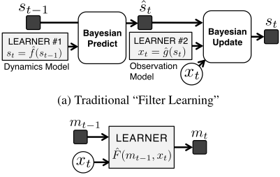
Figure 1: (a) Traditional learning-based methods decouple the filter-learning problem to that of learning separate models for the transition and observation functions that can be be later used for the inference procedure (Bayesian filtering). (b) Inference Machines optimize for inference performance by directly learning a filter function that predicts the next belief state mt given the previous belief state mt-1 and the current observation xt. Our discriminative approach combines the predict and update steps and allows us to utilize powerful learning algorithms to learn more accurate filters.
In many domains, such as robotics, it becomes difficult to robustly characterize the dynamics and sensor (observation) physics a priori with simple analytic models. As a result, data driven approaches provide an important tool: they allow models of noisy, complicated dynamics to be learned directly from a robot's interaction with its environment. Learned models can be used for filtering, e.g., the Kalman Filter for linear dynamics and observation models with additive Gaussian noise [Roweis and Ghahramani, 1999], the Unscented Kalman Filter for nonlinear models with Gaussian noise [Wan and Van Der Merwe, 2000], or particle filters for nonlinear models from other distributions [Thrun et al., 2005]. The benefits and limitations of each of these approaches is wellknown. For example, although the particle filter is capable of representing complex distributions, it has trouble scaling with the dimensionality of the state space. Additionally, errors in the dynamics, sensor, and noise models can compound. The cascading of modeling errors during the predict and update steps can result in poor filtering performance.
(a) Quadrotor Hovering
(b) Kinova Mico Grasping
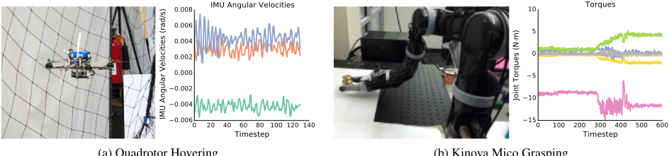
Figure 2: Many real-world systems rely on the ability to utilize observations from noisy sensors in order to update a belief over some component of state. For example, the attitude of a quadrotor from linear accelerations and angular velocities (left) or the mass of a grasped object from the robot's joint positions and applied torques (right).
Likelihood maximization is the natural optimization target for the filtering problem: we wish to determine the most likely sequence of states from a sequence of observations, often on the graphical model structure of a Hidden Markov Model (Fig. 4). Traditional Maximum Likelihood methods attempt to maximize the likelihood of the observations with respect to a specific parametrization describing the graphical model. However, optimizing for the dynamics' model parameters is generally a nonconvex objective due to the cascading structure of time series problems [Abbeel and Ng, 2005]. In this work, we introduce an approach that jointly couples both the process and sensor models by directly optimizing for a filter function that predicts the next belief (Fig. 1b).
We learn the filter function by leveraging ideas from inference machines [Langford et al., 2009; Bagnell et al., 2010; Ross et al., 2011b]. An inference machine is a supervised learning approach developed for learning message passing procedures in probabilistic graphical models. Instead of separating the inference problem (e.g. filtering) from the model learning, inference machines directly reduce the problem of learning graphical models to solving a set of supervised learning problems. We specialize inference machines for two settings: the supervised-state setting and the latent-state setting.
In the supervised-state setting, we wish to learn a filter model for a system with a known state representation for which we are able to obtain ground truth at training time. For example, filtering for a simple pendulum (mass on string) dynamical system in this formulation may use a sufficient-state representation of the angle and velocity (✓↪ ˙ ✓) with observations of the pendulum's Cartesian x position. Note that at test time, we do not assume access to the state values and instead infer them by filtering on observations.
The supervised-state setting contrasts with the latent-state setting in that the sufficient underlying state representation is at least partially unobserved at training time. In the pendulum example, if the system state is parametrized by only ✓, then the representation would be insufficient to predict future states and observations. This partial-parametrization may be a result of any inability to collect training data of the full state at training time or we may not know the full representation of the underlying state. To address this setting, we extend PREDICTIVE STATE INFERENCE MACHINES (PSIMS) [Sun et al., 2015] to exploit any partial-parametrization or sideinformation of state, which we denote as "Hints" about the state.
Concretely, the original PSIMS address prediction over the space of future observations. Many real world applications, however, require the estimation or prediction of useful physical quantities, which traditional filtering algorithms are capable of but PSIMS were not. Our extension, PSIM+HINTS, adds this vital capability, allowing PSIMS to be used in a wide range of filtering application domains including neural signal decoding for prosthetic control, visual tracking where a bounding-box must be predicted, and robot localization. The estimated physical quantities in each domain are the Hints we aim to predict in our framework.
In contrast with the learning literature for system identification, which focuses on learning state representations and corresponding transition and observation models, this work focuses on the filtering or inference task where the observer is maintaining a belief about the current state of the system. We present PREDICTIVE STATE INFERENCE MACHINES WITH HINTS (PSIMS+HINTS) to directly target the inference task of filtering on latent-state space models. As a special case of PSIM+HINTS, we develop the INFERENCE MACHINE FILTER (IMF) for the supervised-state graphical model. Both procedures learn a filter function that uses the current belief state and latest observation to predict the next belief state. The algorithms that we present for learning these inference machines are easy to implement, data-efficient, make no assumptions on the differentiability of the underlying learners, and give theoretical guarantees on the inference task.
2 Inference Machines for Latent-State Models
First, we consider the latent-state setting and introduce PREDICTIVE STATE INFERENCE MACHINES (PSIMS). We then describe and analyze our novel addition to this underlying framework, which we call PREDICTIVE STATE INFERENCE MACHINE WITH HINTS (PSIM+HINTS). This allows us to consider a partially-observed state setting and use inference machines for filtering. We then show that PSIM+HINTS can be easily adapted to learn INFERENCE MACHINE FILTERS (IMFS) for the supervised-state setting in Section 3.
2.1 PREDICTIVE STATE INFERENCE MACHINES
The inference machine approach of [Ross et al., 2011b] cannot be applied to learning latent-sate space models since we do not have access to the hidden states' information at training time (versus the supervised-state setting). This difficulty can be overcome by leveraging ideas from Predictive State Representations (PSRs) [Littman et al., 2001; Singh et al., 2004; Boots et al., 2011; Hefny et al., 2015]. In contrast to latent variable representations like HMMs [Siddiqi et al., 2010; Hsu et al., 2012; Song et al., 2010] or linear state space models [Van Overschee and De Moor, 2012], which represent the belief state as a distribution over the latent-state space of the model, PSRs instead maintain an equivalent belief over sufficient features of future observations. Specifically, we assume that there exists a bijective function such that:
With this representation, the PREDICTIVE STATE INFERENCE MACHINE (PSIM) [Sun et al., 2015] uses the predictive state for supervised training in the inference machine framework. More formally, the goal is to learn an operator F that can deterministically pass the predictive states forward in time conditioned on the latest observation,
where ft = [xt+kf ↪ ▷ ▷ ▷ ↪ xt+1] is the sequence of future observations and pt = [xt↪ ▷ ▷ ▷ ↪ x0] is the full history of past observations. We further assume that there exists a bijective mapping from P(ft♣pt) to the conditional expectation E[φ(ft)♣pt] for feature function φ. For example under a Gaussian distribution E [φ(ft)♣pt] = E ⇥f↪ ff T ♣pt ⇤, the sufficient statistics for the distribution.
such that the likelihood of the observations ¶ft♦t generated from the sequence of predictive states ¶E[φ(ft)♣pt]♦t is maximized. As this is is a sequential prediction problem over the predictive states, DAgger [Ross et al., 2011a] is used to optimize the inference machine. The choice of learner for F can be any no-regret regression or classification algorithm.
2.2 PREDICTIVE STATE INFERENCE MACHINE WITH HINTS
In this section, we extend PSIMS to models with partially observable states or side-information (Fig. 3a). This structure shows up in many practical problems. The "Hints" h may be a bounding-box in visual tracking, the decoded command from a brain-computer interface, or the pose of a robot. In this semi-supervised setup, the hints h and observations x are at training time though the true sufficient-state s is either unknown or unobserved. Although PSIM is well defined on a simple chain-structured model (e.g. Fig. 4), it is not straightforward to extend PSIM to a model with the complicated latent structure in Fig. 3a.
To handle this type of graph structure, we collapse the hints h and the latent states s into a single unit-configuration as shown in the abstracted factor graph, Fig. 3b, and only focus on the net message passed into the configuration and the net message passed out from the configuration. Ideally, we would like to design an inference machine that mimics this net message passing procedure.
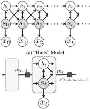
In Fig. 3b, mt represents the joint belief of ht and st,
Directly tracking these messages is difficult due to the existence of latent state st. Following the approach of PSRs and PSIMS, we use observable quantities to represent the belief of ht and st. Since the latent state st affects the future observations starting from xt, and also the future partial states starting from ht, we use sufficient features of the joint distribution of future observations and hints to encode the information of st in message mt-1. Similar to PSIM, we assume that there exists an underlying mapping between the following two representations:
Assuming that φ computes the sufficient features (e.g., first and second moments), we can represent P(ht↪ xt+1:t+kf ♣pt) by the following conditional expectation:
When φ is rich enough, E ⇥φ(ht↪ xt+1:t+kf )♣pt ⇤ is equivalent to the distribution P(ht↪ xt+1:t+kf ♣pt). For example, if φ is a kernel mapping, E ⇥φ(ht↪ xt+1:t+kf )♣pt ⇤ essentially becomes the kernel embedding of P(ht↪ xt+1:t+kf ♣pt). We call E ⇥φ(ht↪ xt+1:t+kf )♣pt ⇤ as the predictive state. For notational simplicity, define mt = E ⇥φ(ht↪ xt+1:t+kf )♣pt ⇤.
Algorithm 1 PSIM+HINTS with DAgger Training
- 1: Input: M independent trajectories ⌧i, 1 i M;
- 3: Initialize F0 to be any hypothesis in F;
- 2: Initialize D D0 ;
- 4: Initialize ˆm1 = 1M PMi=1 φ(hit ↪ f i1 = xi1:k ) 5: for n = 0 to N do
- 7: Create dataset Dn: 8⌧i, add predicted message with observation zi t = ( ˆmi↪Fn t ↪ xit ) encountered by Fn to Dn as feature variables (inputs) and the corresponding φ(hit+1 ↪ f i t+1 ) to Dn as the learning targets ;
- 6: Roll out Fn to performbelief propagation on trajectory ⌧i, 1 i M
- 8: DAgger Step: aggregate dataset, D =D[Dn;
- 9: Train a new hypothesis Fn+1 on Dn to minimize the loss d(F (m↪ x)↪ φ(h↪ f ));
- 10: end for
- 11: Return: Best hypothesis ˆ F 2 ¶Fi♦Ni=0 on validation trajectories.
We are then capable of training an inference machine that mimics the following predictive state flow:
which takes the previous predictive state mt-1 and current observation xt and outputs the next predictive state mt.
Define ⌧ ⇠ D as a trajectory ¶x1↪ h1↪ ▷▷▷↪ xT ↪ ht♦ of observations and hints sampled from an unknown distribution D. Given a function F 2 F, let us define m⌧↪F t as the corresponding predictive state generated by F when rolling out using the observations in ⌧ described by Eq. 6.
Similar to PSIM, we aim to find a good hypothesis F from hypothesis class F, that can approximate the true messages well. Hence, we define the following objective function:
where d is the loss function that measures how good the predictive states are (e.g., the likelihood of (h⌧t ↪ x⌧t+1:t+kf ) being generated from ˆm⌧t or the squared loss).
The optimization objective presented in Eq. 7 is generally nonconvex in F due to the objective involving sequential prediction terms where the output of F from time-step t - 1 is used as the input in the loss for the next timestep t. Often, a simpler surrogate objective function is considered that only optimizes over single-step predictions. However, optimizing the one-step error alone can resulting in cascading errors of O(exp(T)) [Venkatraman et al., 2015]. As optimizing Eq. 7 directly is impractical, we utilize Dataset Aggregation (DAgger) [Ross et al., 2011a] to find a filter function (model) F with bounded error. The training procedure for PSIM+HINTS is detailed in Algorithm 1. By rolling out the learned filter and collecting new training points (lines 6, 7), subsequent models are trained (line 9) to be robust to the induced message distribution caused by sequential prediction.
Specifically, let us define z⌧ t = (h⌧t ↪ x⌧t+1:t+kf ) for any trajectory ⌧ at time step t and define dF as the joint distribution of ( ˆm⌧↪F t-1 ↪ x⌧t ↪ z⌧ t )↪ 8t when rolling out F on trajectory ⌧ sampled from D. Then our objective function can be represented alternatively as E(m↪x↪z)⇠dF d(F(m↪ x)↪ z). Alg. 1 guarantees to output a hypothesis ˆ F such that:
where
which is the minimum batch minimization error from the entire aggregated dataset in hindsight after N iterations of Alg. 1. This result follows by a reduction to DAgger optimization [Ross et al., 2011a] (similar to that in [Venkatraman et al., 2015; Sun et al., 2015]). Note that this bound applies to Eq. 7 for the F found by Alg. 1. Despite the learner's loss ✏ in Eq. 9 being over the aggregated dataset, it can be driven low (e.g. with a powerful learner), making the bound useful in practice. For long-horizons, the possible exponential rollout error from optimizing only the one-step error dominates the error over the aggregated dataset.
We conclude with a few final notes. First, even though F0 would ideally be initialized (line 3) by optimizing for the transition between the true messages, in practice F0 is often initialized from the empirical estimates. Second, though the sufficient-feature assumption is common in the PSR literature [Hefny et al., 2015], an approximate feature transform φ balances computational complexity with prediction accuracy: simple feature design (e.g., first moment) makes for faster training of F while Hilbert Space embeddings are harder to optimize but may improve accuracy [Boots, 2012; Boots et al., 2013]. Additionally, the bound in Eqns. 8, 9 holds for the approximate message statistics. Finally, though the learning procedure is shown in a follow-the-leader fashion on the batch data (line 9), we can use any online no-regret learning algorithm (e.g. OGD [Zinkevich, 2003]), alleviating computational and memory concerns.
Hint Pre-image Computation
Since the ultimate goal is to predict the hint, we need an extra step to extract the information of ht from the computed predictive state ˆmt, which is an approximation of the true conditional distribution P(ht↪ xt+1:t+kf ♣pt). Exactly computing the MLE or mean of ht from ˆmt might be difficult (e.g., sampling points from a Hilbert space embedding is not trivial [Chen et al., 2012]). Instead, we formulate the step of extracting ht from ˆmt as an additional regression step:
To find g, we roll out ˆ F on each trajectory from the training data and collect all the pairs of ˆm⌧t ↪ h⌧t . Then we can use any powerful learning algorithm to learn this pre-image mapping g (e.g., random forests, kernel regression). Note that this is a standard supervised learning problem and not a sequential prediction problem- the output from g is not used for future predictions using g or the filter function ˆ F .
3 The INFERENCE MACHINE FILTER for Supervised-State Models
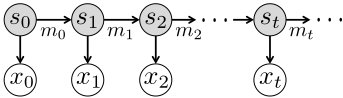
In contrast to filter learning in the latent-state problem, the supervised-state setting affords us access to both the sufficient-state s and observations x during training time. We specifically look at learning a filter function on Hidden Markov Models (HMMs) as shown in Fig. 4. This problem setting similar to those considered in the learningbased system identification literature (e.g. [Ko and Fox, 2009; Nishiyama et al., 2016]). However, these previous methods use supervised learning to learn independent dynamics and observation models and then use these learned models for inference. This approach may result in unstable dynamics models and poor performance when used for filtering and cascading prediction. Instead, we directly optimize filtering performance by adapting PSIM+HINTS to learn message passing in this supervised setting. We term this simpler algorithm as the INFERENCE MACHINE FILTER (IMF).
Referencing Algorithm 1, the IMF simply sets the hints ht in PSIM+HINTS to be the observed states st and sets the number of future observations kf = 0; in other words, st is assumed to be a sufficient-state representation. The IMF learns a deterministic filter function F that combines the predict-and-update steps of a Bayesian filter to recursively compute:
The INFERENCE MACHINE FILTER (IMF) can be viewed as a specialization of both the theory and application of inference machines to the domain of time-series hidden Markov models. Our guarantee in Eq. 8 shows that the prediction error on the messages optimized by DAgger is bounded linearly in the filtering problem's time horizon. Additionally, the sufficient feature representation of PSIM+HINTS allows IMFS to represent distributions over continuous variables, compared to the discrete tabular setting of [Ross et al., 2011b].
The IMF approach differs from [Langford et al., 2009] in several important ways. Langford et al. learn four operators:
one to map the first observation to initial state, one for the belief update with an observation, one for state-to-state transition, and one for state to observation. This results in a more complex learning procedure as well as a special initialization procedure at test time for the filter. Our algorithm only learns a single filter function instead of four. It also operates like a traditional filter; it is initialized from a prior over belief state instead of mapping from the first observation to the first state. Finally, Alg. 1 does not assume differentiability of the learning procedure as required for the backpropagation-throughtime learning used in [Langford et al., 2009].
4 Experiments
We focus on robotics-inspired filtering experiments. In the supervised-state representation, we are given the state (e.g. robot's pose) and observations (e.g. IMU readings) at training time. In the latent-state setting, we only gain access to the observations and instead of observing the full state at training time, we see only a hint (e.g. only the x-position of the pose). In both scenarios, the hint or state could be collected by instrumenting the system at training time (e.g. having the robot in a motion capture arena), which we then do not have access to at test time (e.g. robot moves in an outdoor area). The latent-state setting with hints is additionally relevant in domains where it is difficult to observe the full state but easy to observe quantities that are heavily correlated with it.
4.1 Baselines
We compare our approach against both learning-based algorithms as well as physics based, hand-tuned filters when relevant. For the first baseline, we compare against a learned linear Kalman filter (Linear KF). Here, the hints h are the states X for the Kalman filter and Y are the observations. We learn the Kalman filter using the MAP estimate:
We select the regularization (Gaussian prior) terms β1↪ β2 by cross-validation.
We also compare against a model that uses a fixed-sized history kp of observations to predict the hint at the next time step. We find this model by optimizing the objective,
where ht is the hint we wish to predict at timestep t, yt-kp ↪ ▷ ▷ ▷ ↪ yt are past observations, and AR is the learned function. This baseline is similar to Autoregressive (AR) Models [Wei, 1994]. It is important to note that using a past sequence of observations is different than tracking a belief over the future observations (the predictive state) as PSIM does. The AR model does not marginalize over the whole history as a Bayesian filter would. In our experiments, we set the history (past) length kp = 5. Choosing higher kp reduces the comparability of the results as the AR model has to wait kp timesteps before giving a prediction while the other filter algorithms predict from the first timestep. To get good performance, we chose the AR model to be Random Fourier Features (RFF) regression [Rahimi and Recht, 2007] with hyperparameters tuned via cross-validation.
| Algorithm | Observation Length | Full State Est. s = h ⌘ (✓↪ ˙ ✓) | Partial State Est. s = h ⌘ (✓) |
|---|---|---|---|
| Physics UKF | - | 1▷22 ◦ 1▷2 | N/A |
| AR | kp = 5 | 2▷96 ◦ 1▷5 | 1▷60 ◦ 1▷5 |
| Linear KF | - | 4▷67 ◦ 0▷98 | 1▷81 ◦ 1▷6 |
| IMF | - | 0▷577◦0▷33 | 1▷43◦1▷3 |
| PSIM+HINTS | kf = 5 | 0▷554◦0▷33 | 1▷27◦1▷0 |
| kf = 10 | 0▷549◦0▷32 | 0▷888◦0▷78 | |
| ( kf = 20 | 0.544◦0.31 | 0.758◦0.68 |
Finally, on several of the applicable dynamics benchmarks below, we also compare against a hand-tuned filter for the problem. The overall error is reported as the mean L2 norm error 1 T PTt=1 k ˆ ht - htk2 .
4.2 Dynamical Systems
We describe the experimental setup below for each of the dynamical system benchmarks we use. A simulated pendulum is used to show that the inference machine is competitive with, and even outperforms, a physics-knowledgeable baseline on a sufficient-state representation. This simulated dataset additionally illustrates the power of using predictive state when we only access a partial-state to use as a hint. Two real-world datasets show the applicability of our algorithms on robotic tasks. The numerical results are computed across a k-fold validation (k = 10) over the trajectories in each dataset. We use linear regression or Random Fourier Feature (RFF) regression to learn the message passing function F for PSIM+HINTS and IMF and report the better performing result. Random forests [Breiman, 2001] or RFF regression are used to learn the pre-image map g, chosen by cross-validation over that k-fold's training trajectories.
Pendulum State Estimation
In this problem, the goal is to estimate the sufficient state st = ht = (✓↪ ˙ ✓)t from observations xt of the Cartesian coordinate of the mass at the end of pendulum. For PSIM+HINTS and IMF we use a message that approximates the first two moments. This is accomplished by stacking the state with its element-wise squared value, with the latter approximating the covariance by its diagonal elements. IMF does this for only the state while PSIM+HINTS does this for the hint (state) and the future observations. Since we know the dynamics and observation models explicitly for this dynamical system, we also compare against a baseline that can exploit this domain knowledge, the Unscented Kalman Filter
| Algorithm | Mean L2 Error ◦1σ |
|---|---|
| Complementary Filter | 0▷0167 ◦ 0▷011 |
| AR (kp = 5) | 0▷0884 ◦ 0▷063 |
| Linear KF | 0▷0853 ◦ 0▷066 |
| IMF | 0▷037 ◦ 0▷0305 |
| PSIM+HINTS (kf = 5) | 0.0136 ◦ 0.017 |
(Physics UKF) [Wan and Van Der Merwe, 2000]. The process and sensor models given to the UKF were the exact functions used to generate the training and test trajectories.
Pendulum Partial State Estimation
To illustrate the utility of tracking a predictive state, consider the same simulated pendulum where we take the partial state, ✓t as the hint ht for PSIM+HINTS and use as the (insufficent) state st for the IMF. We use the first and approximate second moment features to generate the messages. On this benchmark, we do not compare against a UKF physics-model since the partial state is not sufficient to define a full process model of the system's evolution.
Quadrotor Attitude Estimation
In this real-world state-estimation problem, we look to estimate the attitude of a quadrotor in hover under external wind disturbance. The quadrotor runs a hover controller in a Vicon capture environment, shown in Fig. 2a. We use the Vicon's output as the ground truth for the roll and pitch of the quadrotor and use the angular velocities and acceleration measurements from an on-board IMU as the observations. As an application specific baseline, we compare against a Complementary Filter [Hamel and Mahony, 2006] hand-tuned by domain experts. We use only first moment features for the messages in PSIM+HINTS and first and approximate second moment features for IMF messages.
| Algorithm | Mean L2 Error ◦1σ |
|---|---|
| AR (kp = 5) | 42▷82 ◦ 19▷62 |
| Linear KF | 89▷13 ◦ 52▷22 |
| PSIM+HINTS (kf = 40) | 32.77 ◦ 14.09 |
Mass Estimation from Robot Manipulator
This dataset tests the filter performance at a parameter estimation task where the goal is to estimate the mass carried by the robot manipulator shown in Fig. 2b. Each trajectory has the robot arm lift an object with mass 45g-355g. The robot starts moving at approximately the halfway point of the recorded trajectories. We use as observations the joint angles and joint motor torques of the manipulator. Only first moment features are used for the messages for PSIM+HINTS. With this experiment, we show that that filtering helps reduce error compared to using simply a sequence of past observations (AR baseline) even on a problem of estimating a parameter held static per test trajectory.
5 Discussion &Conclusion
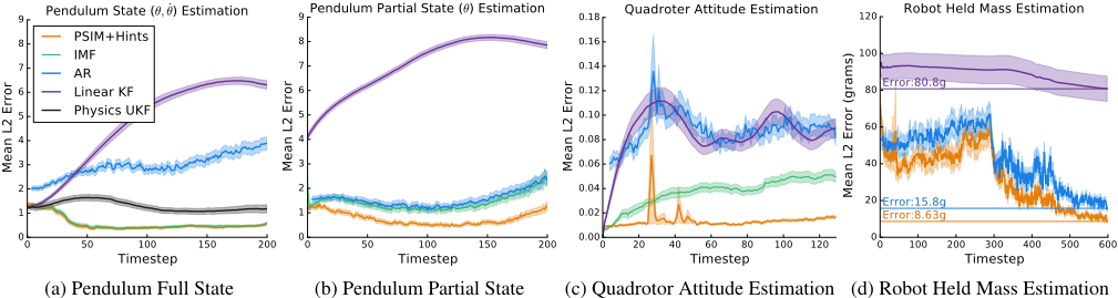
In all of the experiments, IMF and PSIM+HINTS outperform the baselines. Table 1 (left column) shows that the IMF and PSIM+HINTS both outperform the baseline Unscented Kalman Filter which uses knowledge of the underlying physics and noise models. We do not compare against a learned-model UKF, such as the Gaussian Process-UKF [Ko and Fox, 2009], because any learned dynamics and observation models would be less accurate than the exact ones in our Physics UKF baseline. For fair comparison, the UKF, Linear KF, IMF, and PSIM+HINTS all start with empirical estimates of the initial belief state (note the similar error at the beginning of Fig. 5a). We believe that the IMF and PSIM+HINTS outperforms the Physics UKF for two reasons: (1) Inference machines do not make Gaussian assumptions on the belief updates as the UKF does, (2) The large variance for the UKF (Table 1) shows that it performs well on some trajectories. We qualitatively observed this variance is heavily correlated with the difference between the UKFs initial belief-state evolution and the true states. Our proposed inference machine filter methods instead directly optimize the filter's performance over all of the time-horizon are are thus more robust to the initialization of the filter .
The simulated pendulum example also demonstrates the usefulness of predictive representations. When a sufficient state is used (i.e. (✓↪ ˙ ✓) for the pendulum) for the filter's belief, similar performance is achieved using either IMF or PSIM+HINTS. Table 1's right column (or Fig. 5b) shows that when a partial-state representation is used instead (i.e. (✓)), PSIM+HINTS vastly outperforms IMF. Specifically, we require a larger predictive state representation (larger kf ) over the observation space in order to better capture the evolution of the system. This ablation-style experiment demonstrates the ability of PSIM+HINTS to produce more accurate filters.
Finally, our real-world dataset experiments provide additional experimental validation of inference machines for filtering. Both the IMF and PSIM+HINTS outperform baselines in Table 2. In Fig. 5d, PSIM+HINTS is on average 50% more accurate at the end of the trajectory than the AR baseline; the average error over the whole trajectory is given in Table 3. For this problem, the largest information gain is when the robot starts moving halfway along the trajectory. We see less performance gain from using a filter compared to the AR baseline in this problem as the hint (mass) does not change over time as the state does in pendulum or quadrotor problems. The the error versus time plots in Fig. 5 show the relative stability of the inference machine filters even over large time horizons.
In this work, we presented a novel class of inference machines, PSIM+HINTS, which can leverage powerful discriminative supervised learning algorithms to directly approximate belief propagation for filtering on time-series and dynamical systems. The proposed algorithms show promise in many robotic applications where ground-truth information about state is available during training, for example by overinstrumenting to get the hints or state values during prototyping or calibration. We empirically validated our approaches on several simulated and real world tasks, illustrating the advantage of PSIMS+HINTS and IMFS over previous methods.
Acknowledgments
This material is based upon work supported by: NSF Graduate Research Fellowship Grant No. DGE1252522, NSF CRII Award No. 1464219, NSF NRI Purpose Prediction Award No. 1227234, and DARPA ALIAS contract number HR001115-C-0027. Any opinions, findings, and conclusions or recommendations expressed in this material are those of the author(s) and do not necessarily reflect the views of the National Science Foundation. The authors thank Shervin Javdani & John Yao for assistance in collecting robot data.
@inproceedings{ijcai2016p296,
  title     = {Inference Machines for Nonparametric Filter Learning},
  author    = {Venkatraman, Arun and Sun, Wen and Hebert, Martial and Boots, Byron and Bagnell, J. Andrew},
  booktitle = {Proceedings of the Twenty-Fifth International Joint Conference on
               Artificial Intelligence, {IJCAI-16}},
  publisher = {AAAI Press / International Joint Conferences on Artificial Intelligence},
  editor    = {Subbarao Kambhampati},
  pages     = {2074--2080},
  year      = {2016},
  month     = {7},
  url       = {https://ijcai.org/proceedings/2016/296},
}
TY - CPAPER TI - Inference Machines for Nonparametric Filter Learning AU - Venkatraman, Arun AU - Sun, Wen AU - Hebert, Martial AU - Boots, Byron AU - Bagnell, J. Andrew T2 - Proceedings of the Twenty-Fifth International Joint Conference on Artificial Intelligence, IJCAI-16 PB - AAAI Press / International Joint Conferences on Artificial Intelligence PY - 2016 SP - 2074 EP - 2080 UR - https://ijcai.org/proceedings/2016/296 ER -Copied
Machine-readable versions of this paper, for tools and AI agents:





