
Bayesian Optimization of Partition Layouts for Mondrian Processes
Proceedings of the Twenty-Fifth International Joint Conference on Artificial Intelligence. Pages 2160-2165.
Abstract
The Mondrian process (MP) produces hierarchical partitions on a product space as a kd-tree, which can be served as a flexible yet parsimonious partition prior for relational modeling. Due to the recursive generation of partitions and varying dimensionality of the partition state space, the inference procedure for the MP relational modeling is extremely difficult. The prevalent inference method reversible-jump MCMC for this problem requires a number of unnecessary retrospective steps to transit from one partition state to a very similar one and it is prone to fall into a local optimum. In this paper, we attempt to circumvent these drawbacks by proposing an alternative method for inferring the MP partition structure. Based on the observation that similar cutting rate measures on the partition space lead to similar partition layouts, we propose to impose a nonhomogeneous cutting rate measure on the partition space to control the layouts of the generated partitions — the original MCMC sampling problem is thus transformed into a Bayesian global optimization problem. The empirical tests demonstrate that Bayesian optimization is able to find better partition structures than MCMC sampling with the same number of partition structure proposals.
- [Airoldi et al., 2009] Edoardo M. Airoldi, David M. Blei, Stephen E. Fienberg, and Eric P. Xing. Mixed member- ship stochastic blockmodels. In NIPS, pages 33-40, 2009.
- [Aldous, 1981] David J. Aldous. Representations for par- tially exchangeable arrays of random variables. Journal of Multivariate Analysis, 11(4):581-598, 1981.
- [Auer, 2003] Peter Auer. Using confidence bounds for exploitation-exploration trade-offs. The Journal of Ma- chine Learning Research, 3:397-422, 2003.
- [Butland et al., 2005] Gareth Butland, José Manuel Peregrín-Alvarez, Joyce Li, Wehong Yang, Xiaochun Yang, Veronica Canadien, Andrei Starostine, Dawn Richards, Bryan Beattie, Nevan Krogan, et al. Interaction network containing conserved and essential protein com- plexes in Escherichia coli. Nature, 433(7025):531-537, 2005.
- [Fan et al., 2016] Xuhui Fan, Bin Li, Yi Wang, Yang Wang, and Fang Chen. The Ostomachion process. In AAAI, 2016.
- [Globerson et al., 2007] Amir Globerson, Gal Chechik, Fer- nando Pereira, and Naftali Tishby. Euclidean embedding of co-occurrence data. The Journal of Machine Learning Research, 8:2265-2295, 2007.
- [Green, 1995] Peter J Green. Reversible jump Markov chain Monte Carlo computation and Bayesian model determina- tion. Biometrika, 82(4):711-732, 1995.
- [Hoff, 2008] Peter Hoff. Modeling homophily and stochastic equivalence in symmetric relational data. In NIPS, pages 657-664, 2008.
- [Holland et al., 1983] Paul W. Holland, Kathryn Blackmond Laskey, and Samuel Leinhardt. Stochastic blockmodels: First steps. Social Networks, 5(2):109-137, 1983.
- [Kemp et al., 2006] Charles Kemp, Joshua B. Tenenbaum, Thomas L. Griffiths, Takeshi Yamada, and Naonori Ueda. Learning systems of concepts with an infinite relational model. In AAAI, pages 381-388, 2006.
- [Leskovec and Krevl, 2014] Jure Leskovec and Andrej Krevl. SNAP Datasets: Stanford large network dataset collection. http://snap.stanford.edu/data, June 2014. Link
- [Li et al., 2009] Bin Li, Qiang Yang, and Xiangyang Xue. Transfer learning for collaborative filtering via a rating- matrix generative model. In ICML, pages 617-624, 2009.
- [Lloyd et al., 2012] James Lloyd, Peter Orbanz, Zoubin Ghahramani, and Daniel M. Roy. Random function priors for exchangeable arrays with applications to graphs and relational data. In NIPS, pages 998-1006, 2012.
- [Lovász, 2012] László Lovász. Large networks and graph limits, volume 60. American Mathematical Society, 2012.
- [Miller et al., 2009] Kurt Miller, Michael I. Jordan, and Thomas L. Griffiths. Nonparametric latent feature mod- els for link prediction. In NIPS, pages 1276-1284, 2009.
- [Mockus et al., 1978] Jonas Mockus, Vytautas Tiesis, and Antanas Zilinskas. The application of Bayesian methods for seeking the extremum. Towards Global Optimization, 2:117-129, 1978.
- [Nakano et al., 2014] Masahiro Nakano, Katsuhiko Ishig- uro, Akisato Kimura, Takeshi Yamada, and Naonori Ueda. Rectangular tiling process. In ICML, pages 361-369, 2014.
- [Orbanz and Roy, 2015] Peter Orbanz and Daniel M. Roy. Bayesian models of graphs, arrays and other exchangeable random structures. IEEE Transactions on Pattern Recog- nition and Machine Intelligence, 37:437-461, 2015.
- [Porteous et al., 2008] Ian Porteous, Evgeniy Bart, and Max Welling. Multi-HDP: A non parametric Bayesian model for tensor factorization. In AAAI, pages 1487-1490, 2008.
- [Rasmussen, 2006] Carl E. Rasmussen. Gaussian processes for machine learning. MIT Press, 2006.
- [Roy and Teh, 2009] Daniel M. Roy and Yee Whye Teh. The Mondrian process. In NIPS, pages 1377-1384, 2009.
- [Schmidt et al., 2013] Mikkel N. Schmidt, Tue Herlau, and Morten Mørup. Nonparametric Bayesian models of hi- erarchical structure in complex networks. arXiv preprint arXiv:1311.1033, 2013.
- [Srinivas et al., 2010] Niranjan Srinivas, Andreas Krause, Sham M. Kakade, and Matthias Seeger. Gaussian process optimization in the bandit setting: No regret and experi- mental design. In ICML, 2010.
- [Wang et al., 2011] Pu Wang, Kathryn B. Laskey, Carlotta Domeniconi, and Michael I. Jordan. Nonparametric Bayesian co-clustering ensembles. In SDM, pages 331- 342, 2011.
- [Wang et al., 2015] Yi Wang, Bin Li, Yang Wang, and Fang Chen. Metadata dependent Mondrian processes. In ICML, pages 1339-1347, 2015.
References were extracted automatically from the PDF and may contain errors.
Full text extracted automatically from the PDF; figures, tables and equations may differ. The PDF is the version of record.
1 Introduction
Stochastic block models [Holland et al., 1983] have drawn increasing research interests in recent years [Kemp et al., 2006; Porteous et al., 2008; Airoldi et al., 2009; Li et al., 2009; Nakano et al., 2014; Fan et al., 2016] with applications in link prediction, community discovery, recommender systems, etc. In many scenarios, it is unlikely to know the number of blocks in advance, therefore Bayesian nonparametric models are developed in favour of its flexibility in parameter settings. The infinite relational model (IRM) [Kemp et al., 2006], which imposes a Chinese restaurant process (CRP) on each dimension of the relational data, has demonstrated its practicality for discovering the underlying structure of relational data in regular-grid patterns. The multifurcation Gibbs fragmentation tree (MGFT) [Schmidt et al., 2013] is introduced to model the data with multi-scale structures. A more flexible and parsimonious Bayesian nonparametric block model is the Mondrian process (MP) [Roy and Teh, 2009] relational model, which extends the regular-grid partitions to hierarchical partitions as a kd-tree. The random function priors [Lloyd et al., 2012] further extends the block-style piecewise intensity measure into a continuous intensity measure.
Among these partition structures, we are particularly interested in the relational modeling based on the hierarchical partition structure generated by the MP [Roy and Teh, 2009]. Compared to [Kemp et al., 2006; Lloyd et al., 2012] which have efficient inference methods, the MP partition structure is extremely difficult to infer because the partition structure is recursively generated and the partition state space varies during the inference procedure. The reported inference methods for inferring MP partition structures are all based on the Metropolis-Hastings (MH) sampling family, either using the MH algorithm with various types of proposals (e.g., rotation and scaling) [Roy and Teh, 2009] or the reversible-jump MCMC (RJMCMC) [Green, 1995] for varying dimensionality of the partition space [Wang et al., 2011]. However, for the MH approach there is no clear rule to design proposals; while for the RJMCMC approach, there exist the following drawbacks: (1) It requires a number of unnecessary retrospective steps to transit from one partition state to a very similar partition state (see an example in Figure 2); (2) the sampling procedure is prone to fall into a local optimum. These drawbacks seriously diminish the practicality of the MP.
Based on the observation that similar cutting rate measures on the partition space lead to similar partition layouts, we propose to impose a nonhomogeneous cutting rate measure on the partition space to control the layouts of the generated partitions. To this end, we design a piecewise constant nonhomogeneous rate measure imposed on the partition space, from which we can sample cuts using a very simple strategy. Moreover, the nonhomogeneous rate measure can be represented as a vector in the continuous space so that it can be directly optimized through gradient methods. In this way, we transform the original MCMC sampling problem into a Bayesian global optimization problem. We test the proposed inference method for the MP relational model and find that it is able to find better partition structures than RJMCMC sampling with the same number of partition structure proposals.
The remainder of the paper is organized as follows: We introduce some preliminaries regarding the MP in Section 2. The proposed Bayesian optimization method for inferring MP partition structures is presented in Section 3. In Section 4, we will demonstrate the empirical test results of the MP relational modeling. The paper is concluded in Section 5.
2 Preliminaries
2.1 Stochastic Partitions on Exchangeable Graphs
Many real-world relational data can be represented as graphs (2-arrays). A 2-array R is called separately exchangeable if its joint distribution is invariant to random permutations of rows and columns: (Ri↪j) d= (R⇡(i)⇡0 (j)), where ⇡ and ⇡0 denote two independent random permutations over rows and columns of R, respectively. The stochastic partition process on a graph makes use of such exchangeability by reordering rows and columns of R such that the interaction intensity within the blocks of a partition structure is homogeneous under a certain distribution. The distribution of an exchangeable graph can be characterized by a random function ⇥ : [0↪ 1]2 7! [0↪ 1], which is also called "graphon" [Lov´asz, 2012]. By mapping the row and column indices (⇠i↪ ⌘j) onto [0↪ 1]2 , the observation Ri↪j can be generated by some atomic distribution pR (e.g., Bernoulli distribution for link prediction): Ri↪j ♣⇠i↪ ⌘j ↪ ⇥ ⇠ pR(Ri↪j ♣⇥(⇠i↪ ⌘j )), which is the Aldous-Hoover theorem [Aldous, 1981].
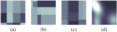
There are a large body of work on Bayesian nonparametric graphons [Orbanz and Roy, 2015], most of which are closely relevant to graph partitions if the underlying graphon is a piecewise constant function. The simplest Bayesian nonparametric graphon is IRM [Kemp et al., 2006], which is constructed by imposing a Chinese restaurant process (CRP) on each side of R, and the resulting graphon is a piecewise constant function with regular grids. Recently, an arbitrarily flexible graphon is proposed which adopts a Gaussian process [Rasmussen, 2006]) as a random graph function prior [Lloyd et al., 2012]. There are also some other Bayesian nonparametric graphons, which sit between the simplicity [Kemp et al., 2006] and the flexibility [Lloyd et al., 2012]. These graphons are constructed in a hierarchical way [Schmidt et al., 2013; Roy and Teh, 2009]; they are not only flexible for modeling complex interactions but also parsimonious for modeling homogeneous parts in R. Some example graphons are illustrated in Figure 1.
2.2 The Mondrian Process Relational Model
Among the above Bayesian nonparametric graphons, the MP [Roy and Teh, 2009] is a typical hierarchical partition process on exchangeable graphs. An MP starts the partition process on the initial block (the unit square [0↪ 1]2 ) with the given budget λ. A trivial cut is first proposed to split the unit square into two blocks, at a cost E. The proposed cut is accepted if λ > E and is rejected otherwise. If accepted, the partition process further steps into the sub-blocks with the rest budget λ -E. The cutting point of each proposal is uniformly sampled from the semi-perimeter of the current block [a↪A] ⇥ [b↪B] and the cost E is exponentially distributed E ⇠ Exp(A - a + B - b). The MP proceeds in such a hierarchical way until the budget is exhausted. The resulting hierarchical partition structure forms a kd-tree on [0↪ 1]2 .
If the intensity measure in each leaf block of an MP partition structure is homogeneous, the resulting graphon is piecewise constant. Suppose the intensity in each leaf block follows a beta distribution for relational modeling, the generative process of the MP relational model is as follows:
where M denotes an MP partition structure, ✓k denotes the intensity in the kth block inM, (⇠i↪ ⌘j) are the indexing variables (locations) of the ith row and the jth column on [0↪ 1]2 , and ✓~(⇠i↪⌘j) maps (⇠i↪ ⌘j) to a leaf block index inM.
2.3 State-of-the-Art Inference Methods
For regular-grid stochastic partition processes such as IRM [Kemp et al., 2006], the inference is straightforward based on Gibbs sampling after integrating out the parameters of the intensity measure on the partitions. For continuous random graph functions such as [Lloyd et al., 2012], with intensity parameters drawn from a Gaussian process, the inference is also tractable due to the existence of Gaussianity in joint, marginal and conditional distributions in the GP [Rasmussen, 2006]. Although the efficient inference problems for IRM and continuous random graph functions have been well addressed, the posterior inference for the MP relational model [Roy and Teh, 2009] is extremely difficult. The generative process of the MP partitions follows a recursive manner, which may require multiple transition steps from one partition state to another similar one; furthermore, the dimensionality of the partition space varies during the inference procedure.
A prevalent method for such dimensionality-varying inference problem is reversible-jump MCMC (RJMCMC) [Green, 1995]. In [Wang et al., 2011], in each partition sampling iteration, a leaf block is selected randomly and a proposal for adding or removing a cut is drawn from a uniform distribution. Then the RJMCMC acceptance ratio is calculated to decide whether the proposed partition structure change is accepted. The above sampling procedure for inferring the MP relational model is inefficient for the following reasons:
- A transition from one suboptimal partition state to another very similar partition state may require multiple

retrospective operations, causing unnecessary high computational cost (see Figure 2).
- The recursive sampling procedure of RJMCMC is prone to converge to local optima, because it is very difficult for the sampler to jump out from a local optimum in a hierarchical state space (compared to a flat state space).
The above limitations diminish the practicality of the MP relational model in real-world applications. It is worth designing an alternative inference method to circumvent them.
3 Bayesian Optimization of Partition Layouts
We attempt to circumvent the limitations aforementioned in Section 2.3 by proposing an alternative method for inferring the hierarchical partition structure for an exchangeable graph. Inspired by the observation that similar cutting rate measures on the partition space lead to similar partition layouts (see examples in Figure 3), we propose to impose a nonhomogeneous rate measure on the partition space to control the layouts of the generated hierarchical partitions. By representing the nonhomogeneous rate measure with a continuouslyvalued vector, we thus make the inference problem feasible for Bayesian optimization. In this way, the original MCMC sampling problem is transformed into an optimization problem in the continuous space of cutting rate measures.
We adopt Bayesian optimization to search the optimal nonhomogeneous rate measure ⇤ , based on which a partition structure S ⇤ is generated in the same way as [Roy and Teh, 2009]. In particular, we view a nonhomogeneous rate measure t and the corresponding likelihood `t of the graph data fitted in the partition structure St generated based on t as the input pair ( t↪ `t) of the Bayesian black-box optimizer (where subscript t denotes the index of the data pairs in the Bayesian optimization). Since the underlying nonhomogeneous rates are continuous values, we can employ a Gaussian process as the surrogate to explore the searching space.
3.1 Nonhomogeneous Cutting Rate Measure
In the MP, the cutting rate is uniform on [0↪ 1]2 (in the 2dimensional case) and the resulting cuts form a homogeneous Poisson process along each dimension parameterized by the budget λ. The expected number of cuts along each side of a rectangle [a↪ A]⇥[b↪ B] is λ(A-a) and λ(B-b), respectively and the expected number of partitions in [a↪A] ⇥ [b↪B] is (λ(A-a)+1)(λ(B-b)+1). This property shows that the density of cuts (or partitions) is uniform on [0↪ 1]2 .
To manipulate the layouts of partitions, we impose a nonhomogeneous rate measure on the partition space, such that the expected number of partitions will be large (or small) in the areas with higher (or lower) cutting rates. A measurable function 1 : [0↪ 1]2 7!R+ can be defined on the unit square and the probability density function of cutting points along the horizontal and vertical axes are

where ¯ (x↪ y) = (x↪ y)◁ R 1 0 R 1 0 (x↪ y)dxdy. The two functions characterize the intensity rates of a nonhomogeneous Poisson process of cutting positions along the horizontal and vertical axes, respectively. Thus, the expected number of cuts along each side of a rectangle [a↪ A] ⇥ [b↪ B] becomes λ R A a R 1 0 ¯ (x↪ y)dxdy and λ R B b R 1 0 ¯ (x↪ y)dxdy.
Based on the above observation, we can generate a desirable partition layouts through controlling the rate measure function ¯ . Although any measurable positive function can be used as the nonhomogeneous rate measure after normalization, we request the nonhomogeneous rate measure to satisfy two properties: (1) It is easy to draw samples from the rate measure function; and (2) The rate measure function is itself simple and can be optimized.
Piecewise Constant Rate Measure We propose to adopt a piecewise constant function defined on [0↪ 1]2 as the nonhomogeneous rate measure. We further let "pieces" of the function be equal-size cells on [0↪ 1]2 such that we can discard the location information and simply represent the function by a set of constants. For example, if we divide [0↪ 1]2 into 3 ⇥ 3 cells and assign each cell a constant as the cutting rate in that cell, the function is thus characterized by a 3 ⇥ 3 matrix (or a 9-D vector). In Figure 3(a), the unit square is divided into 3 ⇥ 3 equal cells, to which are assigned different cutting rates. In the following, we refer to this piecewise constant rate measure as a K ⇥ L "rate matrix" , where K and L denote the numbers of equal intervals along the vertical and horizontal axes, respectively.
Cut Sampling Strategy on Given the piecewise constant rate measure , the probability density functions (2)
1 It is worth noting that the rate measure function and the rate measure matrix defined in this section are conceptually different from the graphons briefed in Section 2.1. The former is the rate measure to generate cuts of a partition structure; while the latter is the rate measure to generate links given a partition structure.
of cutting points along the axes also become piecewise constant. One can sample cuts from different intervals of the axes with different rates; however, there is another simple sampling strategy thanks to such regular-grid piecewise constant measure: Instead of changing cutting rates in different cells, we can still use uniform sampling to achieve the same goal by changing the proportion of each cell on [0↪ 1]2 in terms of their associated cutting rates [Wang et al., 2015]. In particular, we increase (or decrease) the proportion of a cell with higher (or lower) cutting rate on [0↪ 1]2 such that a cut is more likely to fall into the cells with higher rates. After sampling the entire partition structure on the "distorted" partition space, the sampled cuts are mapped back to the original partition space.
Given a K⇥L rate matrix , k↪l denotes the cutting rate in cell (k↪ l). On the original partition space X, the interval of a cell is 1◁K along the vertical axis and 1◁L along the horizontal axis. Then the interval of the "distorted" partition space given can be computed by
The "distorted" partition space ˜ X can be constructed based on ¶δrow k ♦Kk=1 and ¶δcol l ♦Ll=1 (see Figure 3(b,d,f) where the intervals of cells are adjusted according to the cutting rates). The uniformly sampled cuts on ˜ X are mapped back to X by
where (x↪ y) and (˜x↪ ˜ y) denote an endpoint of a cut on X and ˜ X, respectively; k0 and l0 denote the interval indices of the endpoint on the vertical and horizontal axes, respectively.
3.2 Property of the Cutting Rate Matrix
The number of cells in the cutting rate matrix (determined by K and L) can be set as the hyper-parameter. In the following, we first analyze some properties of the cutting rate matrix and then discuss how to set the hyper-parameter.
Property 3.1. The expected number of blocks in an Mondrian process given the same budget λ is irrelevant to the hyperparameter (number of cells) of the cutting rate matrix.
The cutting rate matrix only distorts the original partition space, while the generative process of cuts on the "distorted" partition space is not affected. Thus, the expected number of blocks will be unchanged given the same budget λ.
Property 3.2. Given a fixed number of intervals in one dimension of the cutting rate matrix, increasing the number of intervals in the other dimension will decrease the diversity of the marginal rates in this dimension.
Suppose we have two cutting rate matrices 2 RK⇥L + and 0 2 RK0⇥L + , K > K0 . In our setting, the elements in the cutting rate matrix is drawn from a uniform distribution: k↪l i▷i▷d ⇠ Uniform(0↪ 1). Based on Hoeffding's inequality, the marginal rate PKk=1 k↪l of the lth interval on the horizontal axis for is bounded by Pr(♣ PKk=1 k↪l K - θ♣ ≥ ⌧) exp(-2K⌧ 2 ), where θ = 0▷5 is the expectation of k↪l. The conclusion is straightforward: Given the same tolerance ⌧ and condition K > K0 , the tail bound for the marginal rate is tighter for since exp(-2K⌧ 2 ) < exp(-2K0 ⌧ 2 ), which further implies that the values of marginal rates along the horizontal axis of are less diverse.
Property 3.3. Increasing the numbers of intervals in both dimensions of the cutting rate matrix at the same ratio will first increase and then decrease the diversity of the marginal rates in both dimensions.
Let 2 RK⇥L + and L = ⇢K, ⇢ > 0. Based on Property 3.2, the number of outliers (i.e., the marginal rates outside of (0▷5 - ⌧↪ 0▷5 + ⌧)) in the horizontal dimension of is upper bounded by Lexp(-2K⌧ 2 ) = ⇢K exp(-2K⌧ 2 ). Since the function f(K) = ⇢K exp(-2K⌧ 2 ) is concave in terms of K (first increases and then decreases for K = 1↪ 2↪ ▷ ▷ ▷), its maximum can be derived by solving df(K) dK = ⇢ exp(-2⌧ 2K)(1 - 2⌧ 2K) = 0. Then we can obtain K = round( 1 2⌧ 2 ) that maximizes the upper bound.
Property 3.2 suggests that the diversity of the marginal rates in one dimension can potentially be diminished as the number of intervals in the other dimension increases. Property 3.3 suggests that, to some extend, we are able to manipulate the distortion power of the imposed cutting rate measure on the partition space by tuning the hyper-parameter of the number of cells. In practice, we tune these parameters to achieve the moderate distortion power.
3.3 Cutting Rate Matrix Optimization
Given the imposed nonhomogeneous cutting rate matrix , a partition structure S is first generated based on and then a local Gibbs sampler can be employed to sample the indexing variables ⇠i and ⌘j for all rows and columns in R. Let ` = L(R♣¶⇠i♦↪ ¶⌘j♦↪ S) be the data likelihood based on ; then the pair ( ↪ `) can be used as the input and the reward for Bayesian optimization. The aim of optimizing the underlying partition structure S is to find the maximizer ⇤ that maximizes the reward ` in a sequential manner (see the illustration in Figure 4).
By transforming the MCMC based inference for the MP relational model into an online optimization problem, the following issues need to be considered: (1) The mapping f : 7! ` is unknown; (2) the evaluation of ` given is still expensive, so we cannot exhaustively search the space of ; (3) there exists randomness to generate S based on , thus ` is a noisy observation given . To address these issues, we employ a Bayesian black-box optimizer, without needing to know the explicit formof f : 7! `, to explore the searching space. On one hand, the Bayesian black-box optimizer tends to try that returns higher reward ` with higher probability (exploitation); on the other hand, it still continuously explores unknown space to avoid local optima (exploration).
The empirical reward `t of each St, which is drawn from a given t at the tth iteration, can be obtained by a local Gibbs sampler. We feed a number of pairs ¶ t↪ `t♦ into the proposed Bayesian optimization algorithm. It is worth noting that the uncertainty of St generated based on t can be propagated to the uncertainty `t given f( t). This uncertainty is modeled as the Gaussian noise as

We assume that the similarity over the cutting rate matrix t determines the similarity over the layout of St, and eventually controls the similarity over the expected reward `t. Based on this assumption, the Gaussian process is selected as the surrogate to model f given the covariance matrix over t. The kernel of the GP is constructed by calculating the covariance between t and t0 , which is determined by the metric distance over the cutting rate matrix: cov( t↪ t0) = exp(- 12 ♣♣ t - t0 ♣♣22 ). As the predictive mean and variance are tractable for the GP, a variety of exploitation-exploration strategies for Bayesian optimization can be adopted. Two strategies are adopted in this paper: The first strategy UCB [Srinivas et al., 2010; Auer, 2003] keeps evaluating t that returns the maximum upper confidence bound. The second strategy (EI) [Mockus et al., 1978] selects t that returns the maximum expected improvement (please refer to [Srinivas et al., 2010] for the details). As we essentially choose the optimal partition rather than sampling over multiple partitions, the proposed strategy is different from the MCMC based approach to partition inference (but the generative process of the MP is unchanged).
3.4 The Proposed Algorithm
The proposed algorithm for inferring the MP relational model (whose generative process is described in Section 2.2) in the Bayesian optimization manner is summarized in Algorithm 1. In this algorithm, the outer loop 2 is to search the optimal partition structure S ⇤ based on the proposed Bayesian optimization method while the inner loop employs a local Gibbs sampler for sampling the indexing variables ¶⇠i♦ and ¶⌘j♦ to obtain the data likelihood `t.
Given a cutting rate matrix t in the tth iteration, an exact structure St is generated. The predictive distribution of ¶⇠i♦ and ¶⌘j♦ can be obtained by integrating out the block intensity parameters ¶✓k♦. The conditional posterior of assigning Algorithm 1 Bayesian Optimization for the MP Relational Model
2 It is worth noting that the outer loop is for inferring the partition structure S while the inner loop is for fitting the relational data R given S. The inner loop is same and necessary for all the compared methods considered in Section 4. The empirical test focuses on the comparison of partition structure inference methods (corresponding to the outer loop in Algorithm 1).
Select t using acquisition function (UCB or EI);
Generate St based on t;
Sample the indexing variables ¶⇠i♦ and ¶⌘j♦ according to Eq. (7) using Gibbs sampling;
end for
Evaluate `t based on R↪ St↪ ¶⇠i♦↪ ¶⌘j♦;
end for
Add ( t↪ `t) into the sequence of observation pairs for Bayesian optimization;
Return `⇤ = maxt(`t) and the corresponding S ⇤ .
the ith row to the nth vertical interval on St gives
where δrow n denotes the nth vertical interval of cuts and Sn denotes the set of blocks in St which have interactions with δrow n ; N n↪m i↪+◁- denotes the number of 1 or 0 entries in the ith row of R if it is assigned to the mth block which is crossed by the nth vertical interval; and B(↵0↪ β0) denotes the beta function. The posterior inference for the column indexing variables ¶⌘j♦ is similar to Eq. (7).
4 Experiments
We empirically evaluate the performance of the proposed method and the baseline method for learning the MP relational model on real-world data sets. In particular, we adopt the GPUCB and EI strategies described in Algorithm 1 for the proposed Bayesian optimization approach and the reversiblejump MCMC (RJMCMC) as the baseline. Because of a hierarchical construction of the MP, commonly used inference methods cannot be directly applied. To the best of our knowledge, RJMCMC [Wang et al., 2011] is the only reported and implementable method for the MP. Since our evaluation focuses on the comparison of inference methods for the MP, the proposed method is not compared to other block models or graphons introduced in Section 2.1.
To make fair comparisons, we set the same number of outer iterations, where each outer iteration corresponds to a partition structure change proposal for RJMCMC-MP or a generated partition structure for GPUCB-MP and EI-MP. Within each outer iteration (i.e., each change of the partition structure), 30 iterations (including 20 iterations for burn-in) of Gibbs sampling are conducted for sampling the indexing variables based on the present partition structure. We run 5 individual experiments for all the compared methods (RJMCMCMP, GPUCB-MP, and EI-MP) on each of the data sets.
| HighSchool | NIPS234 | Protein230 | Epinions200 | Slashdot200 | Wikivote200 | |
|---|---|---|---|---|---|---|
| RJMCMC-MP (Log-likelihood) | -1927 | -5588.1 | -5892 | -14649 | -16715 | -14177 |
| RJMCMC-MP (Perplexity) | 1.2686 | 1.1074 | 1.1178 | 1.4423 | 1.5187 | 1.4254 |
| GPUCB-MP (Log-likelihood) | -1928 | -5586.7 | -5796 | -14697 | -16221 | -14046 |
| GPUCB-MP (Perplexity) | 1.2687 | 1.1074 | 1.1158 | 1.4440 | 1.5001 | 1.4207 |
| EI-MP(Log-likelihood) | -1925 | -5756 | -5881 | -13994 | -16332 | -14133 |
| EI-MP(Perplexity) | 1.2683 | 1.1149 | 1.1134 | 1.4189 | 1.5043 | 1.4238 |
We adopt the logarithm of likelihood (Log-likelihood) and the Perplexity as the evaluation metric to measure the performance. A higher log-likelihood or a lower perplexity indicates a better fitness of the data in the inferred graphon. We use the same budget λ = 2 for all the compared methods in all the experiments. For the hyper-parameters of the block intensity, we set ↵0 = 1 and β0 = 1. The cutting rate matrix for the initialization step in GPUCB-MP and EI-MP are randomly generated by k↪l ⇠ Uniform(0↪ 1). Based on its properties discussed in Section 3.2, we set the dimensionality of the cutting rate matrix as 3 ⇥ 3 to achieve a moderate distortion power (see Property 3.2 and 3.3). For RJMCMC-MP, 400 outer iterations (accepted structure change proposals) are conducted; while for GPUCB-MP and EI-MP, 100 outer iterations are conducted for initialization and 300 outer iterations are conducted for prediction.
4.1 Data Sets
We adopt six real-world relational data sets, including 3 directed graphs and 3 undirected graphs, for testing.
Undirected Graphs: The HighSchool (HS) data set consists of 90 students with 269 edges. The NIPS234 (N234) co-author network is generated from the NIPS 1-17 conferences [Globerson et al., 2007] by selecting the top 234 authors in terms of the number of their publications. There are 598 edges in this data set. The Protein230 (P230) network [Butland et al., 2005] describes the relationships among 230 proteins with 595 interactions. The above three data sets have been extensively used for link prediction [Hoff, 2008; Miller et al., 2009; Lloyd et al., 2012].
Directed Graphs: The adopted three preprocessed data sets Epinions200 (E200), Slashdot200 (S200) and Wikivote200 (W200) are from [Leskovec and Krevl, 2014] 3 . The Epinions data set represents who-trust-whom relationships in the social network of the Epinions website. Slashdot is a news website that features new stories on science and technology, which are submitted and rated by its genuine users. The Wikivote data set is the who-votes-on-whom network on the Wikipedia. We adopt a subset of each data set by selecting the top 200 users (the same selection rule as [Globerson et al., 2007] 4 ) in terms of the number of their connected users.
4.2 Results
The comparison results are reported in Table 1. First of all, we can find that the proposed Bayesian optimization based methods, GPUCB-MP and EI-MP, outperform the baseline RJMCMC-MP on all the six data sets. In particular, GPUCB-MP achieves a clear performance gain on Protein230, Slashdot200, and Wikivote200, compared to RJMCMC-MP; while the performance of EI-MP is remarkably better than RJMCMC-MP on Epinions200. The performance of all the three methods are comparable on HighSchool, although EI-MP performs slightly better than RJMCMC-MP. These observations from the results suggest that, under the same computational complexity, the proposed Bayesian optimization based methods can uncover a better partition structure than the RJMCMC based method in most cases.
3 http://snap.stanford.edu/data
4 http://chechiklab.biu.ac.il/gal/data.html
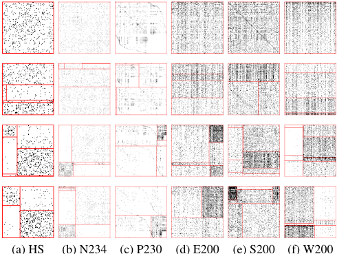
The best inferred partition structures by each method among 5 runs in terms of log-likelihood/perplexity are visualized in Figure 5. On NIPS234, Protein230, Epinions200, Slashdot200 and Wikivote200, the block structures uncovered by GPUCB-MP and EI-MP are significantly interpretable than those uncovered by RJMCMC-MP. The only exception is HighSchool, the block structures uncovered by all the three methods are similar.
5 Conclusion
We propose an alternative method for inferring the MP partition structure by imposing a nonhomogeneous cutting rate measure on the partition space to manipulate the layouts of the generated partitions. By representing the nonhomogeneous cutting rate measure as a simple cutting rate matrix in the continuous space, we can thus transform the original MCMC sampling problem into a Bayesian optimization problem. The experimental results demonstrate that the problem conversion from MCMC sampling to Bayesian optimization helps to explore the partition structure state space more effectively in inferring the Mondrian process relational model. The idea of the proposed Bayesain optimization strategy can also be applied to other complex graphons such as the rectangular tiling process (RTP) [Nakano et al., 2014] by optimizing the growth probabilities in different blocks to manipulate the expected sizes of rectangles.
Acknowledgments
The authors would like to thank the anonymous reviewers for their valuable comments.
@inproceedings{ijcai2016p308,
  title     = {Bayesian Optimization of Partition Layouts for Mondrian Processes},
  author    = {Wang, Yi and Li, Bin and Fan, Xuhui and Wang, Yang and Chen, Fang},
  booktitle = {Proceedings of the Twenty-Fifth International Joint Conference on
               Artificial Intelligence, {IJCAI-16}},
  publisher = {AAAI Press / International Joint Conferences on Artificial Intelligence},
  editor    = {Subbarao Kambhampati},
  pages     = {2160--2165},
  year      = {2016},
  month     = {7},
  url       = {https://ijcai.org/proceedings/2016/308},
}
TY - CPAPER TI - Bayesian Optimization of Partition Layouts for Mondrian Processes AU - Wang, Yi AU - Li, Bin AU - Fan, Xuhui AU - Wang, Yang AU - Chen, Fang T2 - Proceedings of the Twenty-Fifth International Joint Conference on Artificial Intelligence, IJCAI-16 PB - AAAI Press / International Joint Conferences on Artificial Intelligence PY - 2016 SP - 2160 EP - 2165 UR - https://ijcai.org/proceedings/2016/308 ER -Copied
Machine-readable versions of this paper, for tools and AI agents:





