
Preference Inference through Rescaling Preference Learning
Proceedings of the Twenty-Fifth International Joint Conference on Artificial Intelligence. Pages 2203-2208.
Abstract
One approach to preference learning, based on linear support vector machines, involves choosing a weight vector whose associated hyperplane has maximum margin with respect to an input set of preference vectors, and using this to compare feature vectors. However, as is well known, the result can be sensitive to how each feature is scaled, so that rescaling can lead to an essentially different vector. This gives rise to a set of possible weight vectors - which we call the rescale-optimal ones - considering all possible rescalings. From this set one can define a more cautious preference relation, in which one vector is preferred to another if it is preferred for all rescale-optimal weight vectors. In this paper, we analyse which vectors are rescale-optimal, and when there is a unique rescale-optimal vector, and we consider how to compute the induced preference relation.
- [Aizerman et al., 1964] A. Aizerman, E. M. Braverman, and L. I. Rozoner. Theoretical foundations of the potential function method in pattern recognition learning. Automa- tion and Remote Control, 25:821-837, 1964.
- [Ben-Hur and Weston, 2010] Asa Ben-Hur and Jason We- ston. A users guide to support vector machines. In Oliviero Carugo and Frank Eisenhaber, editors, Data Mining Tech- niques for the Life Sciences, volume 609 of Methods in Molecular Biology, pages 223-239. Humana Press, 2010.
- [Brafman and Domshlak, 2009] Ronen I. Brafman and Carmel Domshlak. Preference handling -an introductory tutorial. AI Magazine, 30(1):58-86, 2009.
- [Brafman, 2008] Ronen I Brafman. Preferences, planning and control. In KR, pages 2-5, 2008.
- [Burges, 1998] Christopher JC Burges. A tutorial on support vector machines for pattern recognition. Data mining and knowledge discovery, 2(2):121-167, 1998.
- [Fürnkranz and Hüllermeier, 2010] Johannes Fürnkranz and Eyke Hüllermeier. Preference learning. Springer, 2010.
- [Greco et al., 2010] Salvatore Greco, Vincent Mousseau, and Roman Slowinski. Multiple criteria sorting with a set of additive value functions. European Journal of Opera- tional Research, 207(3):1455-1470, 2010.
- [Herbrich et al., 1999] Ralf Herbrich, Thore Graepel, and Klaus Obermayer. Support vector learning for ordinal re- gression. In Artificial Neural Networks, 1999. ICANN 99. Ninth International Conference on (Conf. Publ. No. 470), volume 1, pages 97-102. IET, 1999.
- [Joachims, 2002] Thorsten Joachims. Optimizing search en- gines using clickthrough data. In Proceedings of the eighth ACM SIGKDD international conference on Knowledge discovery and data mining, pages 133-142. ACM, 2002.
- [Kazawa et al., 2005] Hideto Kazawa, Tsutomu Hirao, and Eisaku Maeda. Order svm: a kernel method for order learning based on generalized order statistics. Systems and Computers in Japan, 36(1):35-43, 2005.
- [Marinescu et al., 2012] Radu Marinescu, Abdul Razak, and Nic Wilson. Multi-objective influence diagrams. In Un- certainty in Artificial Intelligence (UAI), pages 574-583, 2012.
- [Marinescu et al., 2013] Radu Marinescu, Abdul Razak, and Nic Wilson. Multi-objective constraint optimization with tradeoffs. In Proc. CP-2013, pages 497-512, 2013.
- [Montazery and Wilson, 2016] Mojtaba Montazery and Nic Wilson. Learning user preferences in matching for ridesharing. In Proceedings of the 8th International Con- ference on Agents and Artificial Intelligence (ICAART 2016), volume 2, pages 63-73, 2016.
- [Stolcke et al., 2008] Andreas Stolcke, Sachin Kajarekar, and Luciana Ferrer. Nonparametric feature normalization for svm-based speaker verification. In Acoustics, Speech and Signal Processing, 2008. ICASSP 2008. IEEE Inter- national Conference on, pages 1577-1580. IEEE, 2008.
- [Trabelsi et al., 2011] Walid Trabelsi, Nic Wilson, Derek Bridge, and Francesco Ricci. Preference dominance rea- soning for conversational recommender systems: a com- parison between a comparative preferences and a sum of weights approach. International Journal on Artificial In- telligence Tools, 20(4):591-616, 2011.
- [Wilson and Montazery, 2016] Nic Wilson and Mojtaba Montazery. Preference Inference Through Rescaling Preference Learning (extended version of current pa- per including proofs). Available at http://ucc.insight- centre.org/nwilson/RescalingProofs.pdf, 2016. Link
- [Wilson et al., 2015] Nic Wilson, Anne-Marie George, and Barry O'Sullivan. Computation and complexity of pref- erence inference based on hierarchical models. In Proc. IJCAI-2015, 2015. IJCAI
- [Wilson, 2014] Nic Wilson. Preference inference based on lexicographic models. In Proc. ECAI-2014, pages 921- 926, 2014.
References were extracted automatically from the PDF and may contain errors.
Full text extracted automatically from the PDF; figures, tables and equations may differ. The PDF is the version of record.
1 Introduction
In many contemporary application domains, for example, information retrieval from large databases or the web, or planning in complex domains, the user has little knowledge about the set of possible solutions or feasible items, and what they generally seek is the best that's out there. But since the user does not know what is the best achievable, they typically cannot characterize it or its properties specifically [Brafman, 2008]. So, it is desirable for the system to learn the user's preferences over alternative choices (that is, documents, movies, products and so on) [Brafman and Domshlak, 2009].
Generally, a preference learning task consists of some set of items for which preferences are known, and the task is to learn a function which predicts preferences for a new set of items. An established approach to modeling preferences makes use of the concept of a utility function. Such a function assigns an abstract degree of utility to each alternative under consideration [F¨urnkranz and H¨ullermeier, 2010]. Learning a utility function from a given set of training data could be viewed from a machine learning perspective. However, training data is not necessarily given in the form of input/output pairs, but may consist of qualitative feedback in the form of pairwise comparisons, stating that one alternative is preferred to another one and therefore has a higher utility degree. Support Vector Machine (SVM) approaches [Burges, 1998] are popular in machine learning, and have inspired the development of several methods for preference learning, such as OrderSVM [Kazawa et al., 2005], SVOR [Herbrich et al., 1999] and SVMRank [Joachims, 2002]. Essentially, SVM-based methods are built under this assumption that the utility function is a linear weighted sum of the features. Despite the fact that a linear structure for the preference function may sound too restrictive, incorporating the kernel trick [Aizerman et al., 1964] alleviates this by providing more flexibility, to model non-linear functions as well.
Feature spaces normalization (scaling) is an essential requirement for any SVM-based method because they are not invariant to the scale of their input feature spaces: multiplying a feature dimension by a fixed constant > 1 gives that dimension more weight in the value of the SVM objective function and, therefore, in the choice of the weight vector in the preferences function [Stolcke et al., 2008; Ben-Hur and Weston, 2010]. If we base the scalings on the input instances, then it can make the induced preference relation sometimes highly sensitive to precisely which instances are received. There can thus be subjective, and even rather arbitrary, choices in the scaling of the feature spaces; different ways lead to different preference relations. This suggests defining a more cautious preference relation, consisting of all pairs that are inferred for all choices of scalings.
Thus, one alternative is preferred to another if it is preferred for all rescale-optimal weight vectors, where the rescale-optimal vectors are those that can be made optimal for some rescaling. This is a form of preference inference; a related form is when we only keep preferences that are supported by all compatible weight vectors, which corresponds to the kind of preference inference considered in [Marinescu et al., 2013]. Other forms of preference inference, based on more qualitative, lexicographic, models are considered in [Trabelsi et al., 2011; Wilson, 2014; Wilson et al., 2015]. Other preference reasoning techniques based on a family of utility functions include e.g., [Greco et al., 2010].
In this paper we analyse the new preference relation, deriving results regarding rescale-optimality that entail when scaling makes a difference, and that lead to a characterisation that allows computation of preference.
Section 2 defines the preference relation, and the notion of rescale-optimality, and gives some basic properties. It can happen that rescaling makes no difference; we show how to determine this in Section 3. In Sections 4 and 5 we give characterisations for rescale-optimality, that lead to a way of computing the relation, which we test out with benchmarks derived from a real ride-sharing dataset in Section 6.
2 RescaledMaximumMargin Preference Learning
In this section we define, and give some properties of, a preference relation based on rescaling maximum margin preference learning.
2.1 Some Terminology
We first list some terminology that we'll be using throughout the paper. Consider arbitrary u↪ v↪ w 2 IRn . We say that v is non-zero if v is not equal to the zero vector 0 = (0↪ ▷ ▷ ▷ ↪ 0) 2 IRn . Also, v is said to be strictly positive if v(j) > 0 for all j = 1↪ ▷ ▷ ▷ ↪ n; let IRn+ be the set of strictly positive elements in IRn .
The dot product u · v is equal to Pnj=1 u(j)v(j). The (Euclidean) norm ♣u♣ of u is given by ♣u♣2 = Pnj=1 (u(j))2 , which equals u · u. We also define u ⊙ v to be the vector in IRn given by pointwise multiplication, and thus, for all j = 1↪ ▷ ▷ ▷ ↪ n, (u ⊙ v)(j) = u(j)v(j). Operation ⊙ is commutative, associative and distributes over addition of vectors. An important property is that for any u↪ v↪w 2 IRn (u ⊙ v) · w = v · (u ⊙ w), since they are both equal to Pnj=1 u(j)v(j)w(j). For ⇤ ✓ IRn , define sets ⇤⇤ , ⇤> and ⇤≥1 by ⇤⇤ = ¶w 2 IRn : 8λ 2 ⇤↪w · λ ≥ 0♦; ⇤> = ¶w 2 IRn : 8λ 2 ⇤↪w · λ > 0♦; and
For finite ⇤ ✓ IRn , we define co(⇤) to be the convex cone generated by ⇤, i.e., the set of all vectors in IRn that can be written as Pv2⇤ rvv, where rv are arbitrary non-negative reals. Then co(⇤) is finitely generated (by ⇤). Elements of co(⇤) are said to be positive linear combinations of elements of ⇤. A polyhedron is the intersection of a finite number of closed half-spaces, so is topologically closed and convex and can be written as ¶w 2 IRn : 8i 2 I↪w · λi ≥ ai♦, for finite I, where each λi 2 IRn and ai 2 IR.
2.2 MaximumMargin Preference Relation
We first describe a simple linear SVM-based preference relation, based on Ranking SVM [Joachims, 2002], but only considering consistent inputs. Let ⇤ and ⇥ be finite subsets of IRn . We call ⇤, the preference inputs, and we call ⇥ the constraints. Each input preference λ 2 ⇤ expresses a linear restriction λ · w > 0 on an unknown user weight vector w 2 IRn . For instance, if there are n-features, and the user has told us that they prefer feature vector ↵ to β (where ↵↪ β 2 IRn , each representing the values of the alternative over the n features), then we induce from this that
↵ · w > β · w, i.e., (↵ - β) · w > 0, so we include ↵ - β in ⇤. (This linear weighting assumption is less restrictive than it sounds; for instance, we could form additional features representing e.g., pairwise products of the basic features, enabling a richer representation of the utility function.) The constraints set ⇥ is used for placing general restrictions on w; in particular, for expressing a restriction that higher values of the jth feature are at least as good; this translates to a constraint of the form w(j) ≥ 0, represented by including ej in ⇥, where ej is the jth unit vector, with ej(j) = 1, and ej(k) = 0 for j 6= k.
The feasible set C(⇤↪⇥) is defined to be ⇤> \ ⇥⇤ . We also define G(⇤↪ ⇥) to be ⇤≥1 \ ⇥⇤ . If ⇥ is empty, we may abbreviate G(⇤↪⇥) to G(⇤) (and similarly, for other definitions).
The margin function marg⇤ : C(⇤↪⇥) ! IR is given by marg⇤(w) = minλ2⇤ w·λ ♣w♣ . This is equal to the distance between hyperplaneHw = ¶θ 2 IRn : θ · w = 0♦ and the closest element of ⇤ to Hw. The definition implies that marg⇤(w) > 0 for all w 2 C(⇤↪⇥), since w · λ > 0 for any w 2 ⇤> and λ 2 ⇤. One might view w·λ ♣w♣ as the degree to which w satisfies the preference λ, with the best w being those that satisfy each λ to the greatest degree, i.e., those that maximise marg⇤(w).
For w 2 IRn we define the associated relation >w by, for ↵↪ β 2 IRn , ↵ >w β if and only if w · ↵ > w · β. Note that for any real r > 0, the relation >rw is equal to >w.
Define the preference relation >mm ⇤↪⇥ by, for ↵↪ β 2 IRn , ↵ >mm ⇤↪⇥ β if and only if there exists w with maximum margin in C(⇤↪⇥) such that ↵ >w β. Theorem 1 implies that ↵ >mm ⇤↪⇥ β if and only if ↵ >w(⇤↪⇥) β, where w(⇤↪⇥) is the element in G(⇤↪ ⇥) with minimum norm. 1 Thus, >mm ⇤↪⇥ is close to being a total order, since for any ↵↪ β 2 IRn we have either ↵ >mm ⇤↪⇥ β or β >mm ⇤↪⇥ ↵ or w(⇤↪ ⇥) · (↵ - β) = 0.
Theorem 1 For finite ⇤↪⇥ ✓ IRn , if C(⇤↪⇥) is non-empty then G(⇤↪⇥) is non-empty and there exists a unique element w(⇤↪⇥) in G(⇤↪⇥) with minimum norm. Also, for w 2 C(⇤↪⇥), w maximises marg⇤ within C(⇤↪⇥) if and only if w is a strictly positive scalar multiple of w(⇤↪ ⇥), i.e., there exists r 2 IR with r > 0 such that w = rw(⇤↪ ⇥).
Example 1: Suppose that ⇤ = ¶(2↪-1)↪ (-1↪ 2)↪ ( 15 ↪ 15 )♦ with ⇥ being empty. Then the feasible set C(⇤↪⇥) = ⇤> which equals the set of all w 2 IRn such that 2w(1) > w(2) and 2w(2) > w(1). The set G(⇤↪⇥) = ⇤≥1 is shown in Figure 1(a); it has two extremal points: (3↪ 2) (corresponding to the intersection of the lines 2y -x = 1 and x+y = 5) and (2↪ 3). The point in G(⇤) with minimum norm is (2▷5↪ 2▷5). Theorem 1 implies that the elements in C(⇤↪⇥) with maximum margin are w with w(1) = w(2). For instance, if w = (1↪ 1) then marg⇤(w) = 1 p2 min(1↪ 1↪ 25 ) = p2 5 . The relation >mm ⇤↪⇥ equals >(2▷5↪2▷5), which is the same as >(1↪1). Thus, ↵ >mm ⇤↪⇥ β, i.e., ↵ - β >mm ⇤↪⇥ 0, if and only
1 Because of the space restrictions, not all the proofs could be included. See [Wilson and Montazery, 2016] for missing proofs.
y
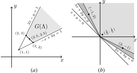
if (↵-β) · (1↪ 1) > 0, i.e., ↵(1)+↵(2)-(β(1)+β(2)) > 0. The set of γ that are >mm ⇤↪⇥ -preferred to 0 is the region in Figure 1(b) to the right of the dotted line.
2.3 The Effect of Rescaling
Consider the effect of a rescaling ⌧, i.e., ⌧ 2 IRn+, where an element v 2 IRn is transformed into v ⊙ ⌧. An input preference vector λ becomes λ ⊙ ⌧ , so ⇤ becomes ⇤ ⊙ ⌧ = ¶λ⊙ ⌧ : λ 2 ⇤♦, and the constraints set ⇥ becomes ⇥⊙ ⌧. The feasible set becomes C(⇤⊙ ⌧↪⇥⊙ ⌧). For example, if ⌧ is the rescaling (1↪ 2) and ⇤ = ¶(2↪-1)↪ (-1↪ 2)↪ ( 15 ↪ 15 )♦ then ⇤ ⊙ ⌧ = ¶(2↪-2)↪ (-1↪ 4)↪ ( 15 ↪ 25 )♦. Rescaling by ⌧ means that each ↵ 2 IRn becomes instead ↵ ⊙ ⌧. Let us say that ↵ is max-margin-preferred to β under rescaling ⌧ if ↵ ⊙ ⌧ >mm ⇤⊙⌧↪⇥⊙⌧ β ⊙ ⌧, i.e., if rescaled ↵ is preferred to rescaled β under the max margin relation relation corresponding to rescaled ⇤ and ⇥. Now, it can easily happen that ↵ is preferred to β under one rescaling, but not under another (see e.g., the example in Section 2.5). Also, the choice of how the features are scaled relative to each other can involve somewhat arbitrary choices. It is therefore natural to consider the relation given by ↵ being preferred to β for all rescalings ⌧ 2 IRn+.
Definition 1 (≫⇤↪⇥) We define relation ≫⇤↪⇥ by, for ↵↪ β 2 IRn , ↵ ≫⇤↪⇥ β if and only if ↵ is max-margin-preferred to β over all rescalings, i.e., if for all ⌧ 2 IRn+, ↵⊙ ⌧ >mm ⇤⊙⌧↪⇥⊙⌧ β ⊙ ⌧ .
Let w⇤ ⌧ (⇤↪ ⇥) (abbreviated to w⇤ ⌧ ) be the element with minimum norm in G(⇤ ⊙ ⌧↪⇥ ⊙ ⌧). Theorem 1 implies that ↵ ⊙ ⌧ >mm ⇤⊙⌧↪⇥⊙⌧ β ⊙ ⌧ if and only if ↵ ⊙ ⌧ >w⇤ ⌧ β ⊙ ⌧, which can be rewritten as ↵ >w⇤ ⌧ ⊙⌧ β.
Defining RO(⇤↪ ⇥) to be ¶w⇤ ⌧ ⊙ ⌧ : ⌧ 2 IRn+♦, we have:
For example, it can be shown that in Figure 1(a), RO(⇤↪⇥) is the closed line segment between (2↪ 3) and (3↪ 2). We show below that RO(⇤↪⇥) is equal the set of rescale-optimal elements in G(⇤↪ ⇥), defined as follows.
Definition 2 (Rescale-optimal) For G ✓ IRn , and u 2 G, let us say that u is rescale-optimal in G if there exists strictly positive ⌧ 2 IRn+ with ♣⌧ ⊙ w♣ ≥ ♣⌧ ⊙ u♣ for all w 2 G.
If 0 2 G then it is the unique element that is rescale-optimal in G. For ⌧ 2 IRn+, we define ⌧ -1 to be the element of IRn+ given by ⌧ -1 (j) = 1◁⌧(j) for all j 2 ¶1↪ ▷ ▷ ▷ ↪ n♦.
Lemma 1 Consider any v 2 IRn and any ⌧ 2 IRn+. Then, v 2 G(⇤↪⇥) if and only if v ⊙ ⌧ 2 G(⇤⊙ ⌧ -1 ↪⇥⊙ ⌧ -1 ). Also, v = w minimises ♣w⊙⌧ ♣ over w 2 G(⇤↪ ⇥) if and only if v = ⌧ -1 ⊙w⇤ ⌧ -1 (⇤↪ ⇥).
Proposition 1 RO(⇤↪⇥) is the set of all rescale-optimal elements of G(⇤↪⇥). Thus, for ↵↪ β 2 IRn , ↵ ≫⇤↪⇥ β if and only if ↵ >w β for all rescale-optimal elements of G(⇤↪⇥), which is if and only if ↵ - β 2 (RO(⇤↪ ⇥))>.
Proof: Consider any v 2 IRn . Then, v is rescale-optimal in G(⇤↪⇥) if and only if there exists ⌧ 2 IRn+ such that v = w minimises ♣w ⊙ ⌧ ♣ over w 2 G(⇤↪ ⇥), which, by Lemma 1, is if and only if there exists ⌧ 2 IRn+ such that v = ⌧ -1 ⊙ w⇤ ⌧ -1(⇤↪⇥), which is if and only if v 2 RO(⇤↪⇥). The last part follows immediately from the definitions. 2
Another natural preference relation ≫⇤⇤↪⇥, which is very closely related to the one explored in [Marinescu et al., 2012; 2013], is given by ↵ ≫⇤⇤↪⇥ β if and only if for all w 2 C(⇤↪⇥), w · (↵ - β) > 0, i.e., iff ↵ is preferred to β for all compatible weight vectors. This holds if and only if for all w 2 G(⇤↪⇥), w · (↵ - β) > 0. Thus, ↵ ≫⇤⇤↪⇥ β if and only if ↵ - β 2 (G(⇤↪⇥))>. (When ⇥ is empty, (G(⇤↪⇥))> is equal to co(⇤), the smallest convex cone containing ⇤.) This implies that if ↵ ≫⇤⇤↪⇥ β then ↵ ≫⇤↪⇥ β. The three defined preference relations are therefore nested: ≫⇤⇤↪⇥ ✓ ≫⇤↪⇥ ✓ >mm ⇤↪⇥ . The three relations are all irreflexive and transitive, and thus strict partial orders (with >mm ⇤↪⇥ close to being a total order). Also, if ≻ is any of the three relations, λ ≻ 0, for any λ 2 ⇤, and for ↵↪ β↪ γ 2 IRn and r 2 IR with r > 0, if ↵ ≻ β then ↵ + γ ≻ β + γ and r↵ > rβ.
2.4 Pointwise Undominated Vectors
For u 2 G(⇤↪⇥), if there exists v 2 G(⇤↪⇥) such that for all j, v(j) is between u(j) and 0 then it is easy to see that u is not rescale-optimal. This is the idea behind being pointwise undominated.
Definition 3 (pointwise dominance) For u↪ v 2 IRn , v pointwise dominates u if u 6= v and for all j 2 ¶1↪ ▷ ▷ ▷ ↪ n♦, either 0 v(j) u(j) or 0 ≥ v(j) ≥ u(j). u is pointwise undominated in G ✓ IRn if there exists no v 2 G that pointwise dominates u.
The definition easily implies that rescale-optimality implies being pointwise undominated.
Proposition 2 Let G ✓ IRn . If u is rescale-optimal in G then u is pointwise undominated in G.
2.5 Example 1 Continued
Since (2▷5↪ 2▷5) has minimum norm in G(⇤), it is rescaleoptimal. The only pointwise undominated elements in G(⇤) are (3↪ 2), (2↪ 3), and the line segment joining them, and, it turns out that all these are rescale-optimal. If we set ⌧ = (r↪ 1) then r p2◁3 will lead to the point (3↪ 2) having minimum value of ♣(x↪ y) ⊙ ⌧ ♣.
Now consider if ⇤ instead equals ¶(2↪ -1)↪ (-1↪ 2)♦. Then G(⇤) has a single extremal point (1↪ 1), being the intersection of the lines 2x - y = 1 and 2y - x = 1. Since (1↪ 1) is the element in G(⇤) with minimum norm, we have w(⇤↪⇥) = (1↪ 1), and (1↪ 1) is rescale-optimal. Thus, >mm ⇤ equals >(1↪1). In fact, (1↪ 1) pointwise dominates every other element in G(⇤), so, by Proposition 2, is the only rescaleoptimal vector in G(⇤). Then, ≫⇤ is just >(1↪1), so that ↵ ≫⇤ β if and only if ↵(x) + ↵(y) > β(x) + β(y). This example shows that allowing rescaling can sometimes make no difference. In Section 3 we show a general result that u is a unique rescale-optimal element in closed convex G if and only if u pointwise dominates every other element of G.
Figure 1(b) illustrates the strength of the three relations, >mm ⇤ , ≫⇤ and ≫⇤⇤, by showing the regions of all γ 2 IR2 that are preferred to 0. For ≫⇤⇤, this is the convex cone generated by the three input vectors ⇤, i.e., all positive linear combinations of them. For ≫⇤, the preferred set is the intersection of the halfspaces ¶γ : γ · (3↪ 2) > 0♦ and ¶γ : γ · (2↪ 3) > 0♦. The largest preference region is associated with >mm ⇤ , with γ >mm ⇤↪⇥ 0 if and only if γ(x) + γ(y) > 0. Since ≫⇤ is not equal to >mm ⇤ , the scaling makes a difference. E.g., (5↪ 0) >mm ⇤ (0↪ 4), which is the same as (5↪ 0) being preferred to (0↪ 4) under rescaling (1↪ 1). However, it can be shown that (0↪ 4) is preferred to (5↪ 0) under rescaling ⌧ = (1↪ 2), with w⇤ ⌧ ⊙ ⌧ being equal to (2↪ 3) (which minimises ♣v ⊙ ⌧ -1 ♣ over v 2 G(⇤)) and (0↪ 4) · (2↪ 3) > (5↪ 0) · (2↪ 3).
3 Determining Uniquely Rescale-Optimal Vectors
Here we characterise the situations when rescaling makes no
difference, i.e., when there is a unique rescale-optimal vector. For convex closed G ✓ IRn , and for ⌧ 2 IRn+ we write
w⌧ (G) for the unique vector w 2 G with minimum value of ♣w ⊙ ⌧ ♣, which makes sense because of the following result. Thus, u is rescale-optimal in convex closed G if and only if there exists ⌧ 2 IRn+ such that u = w⌧ (G).
Lemma 2 Let G be a convex and (topologically) closed subset of IRn . For each strictly positive vector ⌧ 2 IRn+, there exists a unique w 2 G with minimum value of ♣w ⊙ ⌧ ♣.
Theorem 2 below states that u is the only rescale-optimal element in convex closed G if and only if u pointwise dominates every other element of G. The proof uses a pair of lemmas.
Lemma 3 Let u↪ v 2 IRn . There exists k 2 ¶1↪ ▷ ▷ ▷ ↪ n♦ such that ♣u(k)♣ < ♣v(k)♣ if and only if there exists ⌧ 2 IRn+ such that ♣u⊙⌧♣ < ♣v ⊙⌧♣. Thus, for all j 2 ¶1↪ ▷ ▷ ▷ ↪ n♦, ♣u(j)♣ ≥ ♣v(j)♣ if and only if for all ⌧ 2 IRn+, ♣u⊙ ⌧♣ ≥ ♣v ⊙ ⌧♣.
Lemma 4 Let G be a convex subset of IRn , and let j be any element of ¶1↪ ▷ ▷ ▷ ↪ n♦. Then either (i) there exists w 2 G such that w(j) = 0; or (ii) for all w 2 G, w(j) > 0; or (iii) for all w 2 G, w(j) < 0.
Theorem 2 Let G be a convex and closed subset of IRn , and let u be an element of G. Then the following conditions are equivalent.
- (i) u is uniquely rescale-optimal in G, i.e., u is the unique element of G that is rescale-optimal;
- (ii) for all v 2 G, for all j 2 ¶1↪ ▷ ▷ ▷ ↪ n♦, ♣v(j)♣ ≥ ♣u(j)♣;
- (iii) u pointwise dominates every element in G- ¶u♦.
The equivalence between (i) and (ii) is proved using Lemmas 2 and 3, and the equivalence between (ii) and (iii) follows using Lemma 4.
Corollary 1 For finite ⇤↪⇥ ✓ IRn , let G = G(⇤↪⇥). Define y 2 IRn as follows. Choose an arbitrary element z 2 G. For each j 2 ¶1↪ ▷ ▷ ▷ ↪ n♦: If z(j) = 0 then define y(j) = 0. If z(j) > 0 then define y(j) = inf ¶w(j) : w 2 G↪w(j) ≥ 0♦. If z(j) < 0 then define y(j) = sup¶w(j) : w 2 G↪w(j) 0♦. If y 2 G then y is uniquely rescale-optimal in G. Also, there exists a uniquely rescale-optimal element in G if and only if y 2 G.
Corollary 1 leads immediately to an algorithm for determining if G(⇤↪⇥) has a uniquely rescale-optimal element, and finding it, if it exists. The algorithm involves at most n+1 runs of a linear programming solver, and thus determining and finding a uniquely rescale-optimal element u can be performed in polynomial time. If it succeeds in finding such a u then the induced preferences can be efficiently tested using: ↵ ≫⇤↪⇥ β if and only if u · (↵ - β) > 0.
4 Zm-Pointwise Undominated Vectors
Proposition 2 states that being pointwise undominated is a necessary condition for being rescale-optimal. The example below shows that the two conditions are not equivalent. In this section we define a stronger version of pointwise undominated called zm-pointwise undominated, where 'zm' stands for zeros-modified (the essential difference being in the treatment of j such that u(j) = 0). We show that this is still a necessary condition for rescale-optimality, and is in fact equivalent to rescale-optimality (for polyhedra).
Example 2: Let G ✓ IR2 be given by all pairs (x↪ y) such that x + y ≥ 1. It can be seen that the set of points that are pointwise undominated is ¶(x↪ 1-x) : x 2 [0↪ 1]♦. On the other hand, the set of points that are rescale-optimal is ¶(x↪ 1 - x) : x 2 (0↪ 1)♦: neither (1↪ 0) nor (0↪ 1) is rescaleoptimal. This is because if rescaling ⌧ 2 IR2 is such that ⌧(x)◁⌧(y) = r, for r 2 (0↪1), then the associated rescaleoptimal w⌧(G) is equal to 1 1+r2 (1↪ r2 ), which is never equal to (1↪ 0) or (0↪ 1).
Definition 4 (zm-pointwise undominated) We say that u is zm-pointwise undominated in G if for all v 2 G, either (a) v(j) = u(j) for all j 2 ¶1↪ ▷ ▷ ▷ ↪ n♦ such that u(j) 6= 0; or (b) there exists k 2 ¶1↪ ▷ ▷ ▷ ↪ n♦ such that either 0 < u(k) < v(k) or 0 > u(k) > v(k).
It is easily shown that if u is zm-pointwise undominated in convex G then it is pointwise undominated in G. Proposition 3 below shows that being zm-pointwise undominated is a necessary condition for being rescale-optimal. The proof uses the following lemma.
Lemma 5 Let u↪ v 2 IRn , with u 6= v, and let ⌧ 2 IRn+. For δ 2 (0↪ 1] let vδ = δv + (1 - δ)u. Then the following hold:
- (ii) (⌧ ⊙⌧ ⊙u) · (v-u) ≥ 0 if and only if for all δ 2 (0↪ 1], ♣vδ ⊙ ⌧ ♣ > ♣u ⊙ ⌧ ♣.
- (i) For any δ 2 IR, ♣vδ ⊙ ⌧♣2 - ♣u ⊙ ⌧♣2 = δ2 ♣(v - u) ⊙ ⌧ ♣2 + 2δ(⌧ ⊙ ⌧ ⊙ u) · (v - u).
- (iii) There exists ⌧ 2 IRn+ such that (⌧⊙⌧⊙u)·(v-u) ≥ 0 if and only if either (a) v(j) = u(j) for all j 2 ¶1↪ ▷ ▷ ▷ ↪ n♦ such that u(j) 6= 0; or (b) there exists k 2 ¶1↪ ▷ ▷ ▷ ↪ n♦ such that either 0 < u(k) < v(k) or 0 > u(k) > v(k).
Proposition 3 Let u be an element of convex G ✓ IRn . Then:
- (i) u is rescale-optimal in G if and only if there exists ⌧ 2 IRn+ such that for all v 2 G, (⌧ ⊙ ⌧ ⊙ u) · (v - u) ≥ 0.
- (iii) If u is rescale-optimal in G then u is zm-pointwise undominated in G.
- (ii) u is zm-pointwise undominated in G if and only if for all v 2 G, there exists ⌧ 2 IRn+ such that (⌧ ⊙⌧ ⊙u) · (v - u) ≥ 0.
Proof: (i): Using Lemma 2, u is rescale-optimal in G if and only if there exists ⌧ 2 IRn+ such that for all v 2 G- ¶u♦, ♣v ⊙ ⌧ ♣ > ♣u ⊙ ⌧ ♣, which, since G is convex, is if and only if, there exists ⌧ 2 IRn+ such that for all v 2 G-¶u♦ and for all δ 2 (0↪ 1], ♣vδ ⊙⌧♣ > ♣u⊙⌧♣, where vδ = δv +(1-δ)u. By Lemma 5(ii), this is if and only if there exists ⌧ 2 IRn+ such that for all v 2 G - ¶u♦, (⌧ ⊙ ⌧ ⊙ u) · (v - u) ≥ 0, which holds iff for all v 2 G, (⌧ ⊙ ⌧ ⊙ u) · (v - u) ≥ 0.
(ii) By Lemma 5(iii), u is zm-pointwise undominated in G if and only if for all v 2 G- ¶u♦, there exists ⌧ 2 IRn+ such that (⌧ ⊙ ⌧ ⊙ u) · (v - u) ≥ 0, from which (ii) follows. (iii) follows immediately from (i) and (ii). 2
Definition 5 (agreeing on signs) For u↪ v 2 IRn , we say that u and v agree on signs if for all j = 1↪ ▷ ▷ ▷ ↪ n, (i) u(j) = 0 () v(j) = 0; (ii) u(j) > 0 () v(j) > 0; and thus also: (iii) u(j) < 0 () v(j) < 0.
Proposition 3(i) implies the following characterisation of rescale-optimality, by letting θ0 = ⌧ ⊙ ⌧ ⊙ u and θ = θ0 θ0 ·u ; for the converse, we use ⌧ such that θ = ⌧ ⊙ ⌧ ⊙ u, so that ⌧ (j)2 = θ(j)◁u(j) when u(j) 6= 0.
Theorem 3 Consider any u in convex G ✓ IRn . If u = 0 then it is the unique rescale-optimal element of G. Otherwise, u is rescale-optimal in G if and only if there exists θ 2 IRn agreeing on signs with u such that θ·u = 1 and for all w 2 G, θ · w ≥ 1.
It turns out that being zm-pointwise undominated is equivalent to being rescale-optimal, for a polyhedron. (The proof is quite technical, and makes use of classical results about convex sets, see [Wilson and Montazery, 2016].)
Theorem 4 Let u be an element of polyhedron G ✓ IRn . Then, u is rescale-optimal in G if and only if u is zmpointwise undominated in G.
5 Computational Characterisation of Rescale-Optimal
Here we extend the characterisation of rescale-optimality given in Theorem 4, leading to a computational method for testing rescale-optimality, and thus to a method for testing if ↵ ≫⇤↪⇥ β, for ↵↪ β 2 IRn .
5.1 Expressing Rescale-Optimality in Terms of Positive Linear Combinations
Theorem 3 implies that non-zero u is rescale-optimal in G(⇤↪⇥) if and only if there exists a vector θ that agrees on signs with u with θ · w ≥ θ · u for all w 2 G. The main result of this section is the following, that shows that θ is a positive linear combination of certain vectors in ⇤ [ ⇥.
Theorem 5 Let G be a polyhedron, which we write as GI = ¶w 2 IRn : 8i 2 I↪w · λi ≥ ai♦, for finite I, and with each λi 2 IRn and ai 2 IR. Consider any non-zero vector u in GI . Then, u is rescale-optimal in GI if and only if there exists θ 2 IRn that agrees on signs with u such that θ · u = 1 and θ is a positive linear combination of elements of ¶λi : i 2 Ju♦, where Ju = ¶i 2 I : λi · u = ai♦.
Note that this implies that if non-zero u is rescale-optimal in GI then Ju is non-empty, since 0 is the only positive linear combination of the empty set, and θ 6= 0.
The proof uses the following lemmas. We first give a property that follows easily from standard results about convex cones.
Lemma 6 Let ⇤ be a finite subset of IRn and let θ 2 IRn . Then ⇤⇤ ✓ (¶θ♦)⇤ if and only if θ 2 co(⇤).
Lemma 7 Consider non-zero u 2 GI (as defined above). Then u is rescale-optimal in GI if and only if u is rescaleoptimal in GJu = ¶w 2 IRn : 8i 2 Ju↪w · λi ≥ ai♦.
Lemma 8 GJu +¶-u♦ is equal to ¶λi : i 2 Ju♦⇤ .
Proof of Theorem 5
First consider θ 2 IRn such that θ · u = 1. Then it can be seen that ¶w : w · θ ≥ 1♦ + ¶-u♦ = (¶θ♦)⇤ . Also, GJu ✓ ¶w : w · θ ≥ 1♦ if and only if GJu +¶-u♦ ✓ (¶θ♦)⇤ () ¶λi : i 2 Ju♦⇤ ✓ (¶θ♦)⇤ , using Lemma 8, which, by Lemma 6, is if and only if, θ 2 co(¶λi : i 2 Ju♦).
By Lemma 7, u is rescale-optimal in GI if and only if u is rescale-optimal in GJu , which, by Theorem 3, is if and only if there exists θ 2 IRn agreeing on signs with u such that θ·u = 1 and GJu ✓ ¶w : w · θ ≥ 1♦, i.e., θ 2 co(¶λi : i 2 Ju♦), by the earlier argument. 2
We have the following corollary (using the same notation), which shows that testing if u is rescale-optimal in GI can be performed in polynomial time: by first checking that u 2 GI (i.e., for all i 2 I, u · λi ≥ ai), and then testing if a set of inequalities has a solution, using a linear programming solver.
Corollary 2 u is rescale-optimal in GI if and only if u 2 GI and there exists non-negative reals ri for each i 2 Ju, (i.e., i 2 I such that λi · u = ai) and vector ⌧ 2 IRn with for all j 2 ¶1↪ ▷ ▷ ▷ ↪ n♦, ⌧(j) ≥ 1, and ⌧(j)u(j) = Pi2Ju riλi.
5.2 Computation of Inference
For finite subsets ⇤↪⇥ of IRn , and arbitrary ↵↪ β 2 IRn , we would like to be able to determine if ↵ ≫⇤↪⇥ β. Now, ↵ 6≫⇤↪⇥ β if and only if there exists u that is rescale-optimal in G(⇤↪⇥) such that u · (β - ↵) ≥ 0. Labelling ⇤ as ¶λi : i 2 I♦ and ⇥ as ¶✓k : k 2 K♦, it follows, using Theorem 5, that ↵ 6≫⇤↪⇥ β if and only if there exists u 2 IRn and θ 2 IRn , non-negative reals ri for each i 2 I and nonnegative reals sk for k 2 K, such that
- ÷ u · (β -↵) ≥ 0;
- ÷ 8i 2 I, u · λi ≥ 1, and [u · λi = 1 or ri = 0];
- ÷ 8k 2 K, u · ✓k ≥ 0, and [u · ✓k = 0 or sk = 0];
- ÷ 8j = 1↪ ▷ ▷ ▷ ↪ n, u(j) = 0 () θ(j) = 0, and u(j) > 0 () θ(j) > 0; and
6 Experimental Testing
- ÷ θ = Pi2I riλi + Pk2K sk✓k.
The experiments make use of a subset of a year's worth of real ridesharing records, provided by a commercial ridesharing system Carma (see http://carmacarpool.com/). We base our experiments on 13 benchmarks derived from this data-set. Each ridesharing alternative has 7 features, representing different aspects of a possible choice of match for a given user. Each benchmark corresponds to the inferred preferences of a different user. An input preference of alternative ↵i over βi leads to ↵i - βi being included in ⇤. However, a pre-processing phase deletes some elements of ⇤, in order to make it consistent (i.e., ⇤> 6= ;), since in this paper we assume consistent preferences. (We assume no additional constraints, so ⇥ = ;.) More information about the data can be found in [Montazery and Wilson, 2016].
We randomly generate 100 pairs of (↵↪ β), based on a uniform distribution for each feature. A pair (↵↪ β) is called decisive for preference relation ≫⇤ if either ↵ ≫⇤ β or β ≫⇤ ↵ hold, i.e., if ↵ and β are comparable with respect to≫⇤; similarly, for ≫⇤⇤. (All 100 pairs turn out to be decisive for >mm ⇤ , as one would expect.) Table 1 shows the percentage of decisive pairs for ≫⇤ and ≫⇤⇤, as well as the running time per request. CPLEX 12.6.2 is used as the solver on a computer facilitated by a Core i7 2▷60 GHz processor and 8 GB RAM memory. Testing ↵ ≫⇤ β is performed using quite a simple CPLEX model based on the approach in Section 5.2. Determining ↵ ≫⇤⇤ β is based on consistency of a set of linear constraints, so is fast.
The results indicate that for these benchmarks, ≫⇤ is much more decisive than≫⇤⇤. At the same time, ≫⇤ is not equal to the maximum margin relation >mm ⇤ , so, in each case, rescaling makes a difference. Testing preference with respect to ≫⇤ can be performed in reasonable time, the slowest instance being Benchmark 13, with a mean query time of around 5.3 seconds, based on 134 input preferences in ⇤.
| ♣⇤♣ | Decisive Pairs (%) | Time (msec) | |||
|---|---|---|---|---|---|
| ≫⇤ | ≫⇤⇤ | ≫⇤ | ≫⇤⇤ | ||
| 1. | 24 | 19 | 2 | 248 | 9 |
| 2. | 29 | 94 | 0 | 1554 | 7 |
| 3. | 31 | 18 | 0 | 421 | 6 |
| 4. | 36 | 83 | 27 | 2478 | 6 |
| 5. | 38 | 35 | 2 | 2123 | 5 |
| 6. | 41 | 63 | 14 | 3006 | 5 |
| 7. | 53 | 41 | 15 | 873 | 3 |
| 8. | 55 | 97 | 11 | 1347 | 5 |
| 9. | 62 | 54 | 1 | 1218 | 4 |
| 10. | 94 | 62 | 6 | 2810 | 4 |
| 11. | 127 | 67 | 9 | 3495 | 5 |
| 12. | 129 | 77 | 0 | 1652 | 3 |
| 13. | 134 | 68 | 19 | 5330 | 4 |
| Avg | 66 | 60 | 8 | 2217 | 5 |
7 Discussion
We have described a novel way of inducing a preference relation-by considering all possible rescalings when applying a linear SVM-based approach for preference learningand derived formal results that allow its computation. Our experimental results indicate that the relation can be computed in a reasonable time for significantly sized instances, and that the relation can be considerably different from both the maximum margin relation and a simple cone-based relation. The results are also very relevant for a more general situation where one had restrictions on a set of allowable rescalings. There are a number of directions for further work, including: extensions to the case of inconsistent input sets and to the computation of which alternatives among a set can be optimal with respect to some rescaling; analysis-along similar lines as in this paper-to the other natural forms of invariance of feature spaces. Finally, it would be interesting to consider the application and generalisation of our results to other convex optimisation problems.
Acknowledgments
This publication has emanated from research conducted with the financial support of Science Foundation Ireland (SFI) under Grant Number SFI/12/RC/2289. We're very grateful for Carma for the use of their dataset. Thanks to the reviewers for their comments, which helped improve the final version of the paper.
@inproceedings{ijcai2016p314,
  title     = {Preference Inference through Rescaling Preference Learning},
  author    = {Wilson, Nic and Montazery, Mojtaba},
  booktitle = {Proceedings of the Twenty-Fifth International Joint Conference on
               Artificial Intelligence, {IJCAI-16}},
  publisher = {AAAI Press / International Joint Conferences on Artificial Intelligence},
  editor    = {Subbarao Kambhampati},
  pages     = {2203--2208},
  year      = {2016},
  month     = {7},
  url       = {https://ijcai.org/proceedings/2016/314},
}
TY - CPAPER TI - Preference Inference through Rescaling Preference Learning AU - Wilson, Nic AU - Montazery, Mojtaba T2 - Proceedings of the Twenty-Fifth International Joint Conference on Artificial Intelligence, IJCAI-16 PB - AAAI Press / International Joint Conferences on Artificial Intelligence PY - 2016 SP - 2203 EP - 2208 UR - https://ijcai.org/proceedings/2016/314 ER -Copied
Machine-readable versions of this paper, for tools and AI agents:





