
Sparsity Conditional Energy Label Distribution Learning for Age Estimation
Proceedings of the Twenty-Fifth International Joint Conference on Artificial Intelligence. Pages 2259-2264.
Abstract
By observing that the faces at close ages are similar, some Label Distribution Learning (LDL) methods have been proposed to solve age estimation tasks that they treat age distributions as the training targets. However, these existent LDL methods are limited because they can hardly extract enough useful information from complex image features. In this paper, Sparsity Conditional Energy Label Distribution Learning (SCE-LDL) is proposed to solve this problem. In the proposed SCE-LDL, age distributions are used as the training targets and energy function is utilized to define the age distribution. By assigning a suitable energy function, SCE-LDL can learn distributed representations, which provides the model with strong expressiveness for capturing enough of the complexity of interest from image features. The sparsity constraints are also incorporated to ameliorate the model. Experiment results in two age datasets show remarkable advantages of the proposed SCE-LDL model over the previous proposed age estimation methods.
- [Bell and Sejnowski, 1997] Anthony J Bell and Terrence J Sejnowski. The independent components of natural scenes are edge filters. Vision research, 37(23):3327-3338, 1997.
- [Bengio et al., 2001] Yoshua Bengio, Rejean Ducharme, and Pascal Vincent. A neural probabilistic language model. In NIPS, pages 932-938, 2001.
- [Chang et al., 2011] Kuang-Yu Chang, Chu-Song Chen, and Yi-Ping Hung. Ordinal hyperplanes ranker with cost sensi- tivities for age estimation. In CVPR, pages 585-592, 2011.
- [Escalera et al., 2015] Sergio Escalera, Junior Fabian, Pablo Pardo, Xavier Baró, Jordi Gonzàlez, Hugo Jair Escalante, and Isabelle Guyon. ChaLearn 2015 apparent age and cul- tural event recognition: Datasets and results. In ICCV, ChaLearn Looking at People workshop, 2015.
- [Fu and Huang, 2008] Yun Fu and Thomas S Huang. Hu- man age estimation with regression on discriminative ag- ing manifold. ICME, pages 578-584, 2008.
- [Fu et al., 2007] Yun Fu, Ye Xu, and Thomas S Huang. Es- timating human age by manifold analysis of face pictures and regression on aging features. In ICME, pages 1383- 1386, 2007.
- [Geng et al., 2006] Xin Geng, Zhi-Hua Zhou, Yu Zhang, Gang Li, and Honghua Dai. Learning from facial aging patterns for automatic age estimation. In ACM MM, pages 307-316, 2006.
- [Geng et al., 2007] Xin Geng, Zhi-Hua Zhou, and Kate Smith-Miles. Automatic age estimation based on facial aging patterns. TPAMI, 29(12):2234-2240, 2007.
- [Geng et al., 2013] Xin Geng, Chao Yin, and Zhi-Hua Zhou. Facial age estimation by learning from label distributions. TPAMI, 35(10):2401-2412, 2013.
- [Geng, 2016] Xin Geng. Label distribution learning. IEEE Transactions on Knowledge and Data Engineering(IEEE TKDE), in press, 2016.
- [Guo and Mu, 2011] Guodong Guo and Guowang Mu. Si- multaneous dimensionality reduction and human age es- timation via kernel partial least squares regression. In CVPR, pages 657-664, 2011.
- [Guo et al., 2009] Guodong Guo, Guowang Mu, Yun Fu, and Thomas S Huang. Human age estimation using bio- inspired features. In CVPR, pages 112-119, 2009.
- [Hinton, 1986] Geoffrey E. Hinton. Learning distributed rep- resentations of concepts. In Cognitive Science Society, pages 1-12, 1986.
- [Lanitis et al., 2002] Andreas Lanitis, J Taylor, Chris, and Timothy F Cootes. Toward automatic simulation of aging effects on face images. TPAMI, 24(4):442-455, 2002.
- [Lanitis et al., 2004] Andreas Lanitis, Chrisina Draganova, and Chris Christodoulou. Comparing different classi- fiers for automatic age estimation. IEEE Transaction on Systems, Man, and Cybernetics, Part B: Cybernetics, 34(1):621-628, 2004.
- [LeCun and Huang, 2005] Yann LeCun and Fu Jie Huang. Loss functions for discriminative training of energy-based models. In AISTATS, 2005.
- [Lee et al., 2006] Honglak Lee, Alexis Battle, Rajat Raina, and Andrew Y Ng. Efficient sparse coding algorithms. In Advances in neural information processing systems, pages 801-808, 2006.
- [Mathias et al., 2014] Markus Mathias, Rodrigo Benenson, Marco Pedersoli, and Luc Van Gool. Face detection with- out bells and whistles. In ECCV, pages 720-735, 2014.
- [Olshausen and others, 1996] Bruno A Olshausen et al. Emergence of simple-cell receptive field properties by learning a sparse code for natural images. Nature, 381(6583):607-609, 1996.
- [Osindero et al., 2006] Simon Osindero, Max Welling, and Geoffrey E Hinton. Topographic product models ap- plied to natural scene statistics. Neural Computation, 18(2):381-414, 2006.
- [Poultney et al., 2006] Christopher Poultney, Sumit Chopra, Yann L Cun, et al. Efficient learning of sparse representa- tions with an energy-based model. In Advances in neural information processing systems, pages 1137-1144, 2006.
- [Ricanek Jr and Tesafaye, 2006] Karl Ricanek Jr and Tami- rat Tesafaye. Morph: A longitudinal image database of normal adult age-progression. In FGR, pages 341-345, 2006.
- [Schwenk and Gauvain, 2002] Holger Schwenk and Jean- Luc Gauvain. Connectionist language modeling for large vocabulary continuous speech recognition. In ICASSP, pages 765-768, 2002.
- [Sun et al., 2013] Yi Sun, Xiaogang Wang, and Xiaoou Tang. Deep convolutional network cascade for facial point detection. In CVPR, pages 3476-3483, 2013.
- [Yan et al., 2007] Shuicheng Yan, Dong Xu, Benyu Zhang, HongJiang Zhang, Qiang Yang, and Lin Stephen. Graph embedding and extensions: A general framework for di- mensionality reduction. TPAMI, 29(1):40-51, 2007.
References were extracted automatically from the PDF and may contain errors.
Full text extracted automatically from the PDF; figures, tables and equations may differ. The PDF is the version of record.
1 Introduction
In recent years, a huge number of research about age estimation has been done because of its potential applications, e.g., Human Computer Interaction (HCI) [Geng et al., 2006], face recognition [Lanitis et al., 2002] or security control [Guo et al., 2009].
In the past few years, some age estimation methods have been proposed. To name a few, Lanitis et al. [Lanitis et al., 2002; 2004] exploited a quadratic function called aging function to predict the ages from facial images. Geng et al. [Geng et al., 2006; 2007] developed AGES algorithm which is based on the subspace trained on a data structure called aging pattern vector. Then, multiple linear regression was used to solve the age estimation problem in [Fu and Huang, 2008; Fu et al., 2007]. Guo et al. used Biologically Inspired Features (BIF) [Guo et al., 2009] and Kernel Partial Least Squares (KPLS) regression [Guo and Mu, 2011] for age estimation. Later, Chang et al. [Chang et al., 2011] transformed an age estimation task into multiple cost-sensitive binary classification subproblems, and solved the problem with an Ordinal Hyperplane Ranking (OHRank) algorithm.
⇤Corresponding author
After that, Geng et al.observed that the faces at close ages look similar since aging is a slow and smooth process, so one face image can also contribute to the learning of its adjacent ages. Inspired by this observation, they proposed Label Distribution Learning (LDL) [Geng et al., 2013], in which an age distribution is assigned to each face image as the training target instead of an age alone, to solve age estimation task. Thus, compared with single label methods, LDL can exploit a dataset more sufficiently. In the following years, some LDL methods were proposed, such as IIS-LDL, CPNNLDL [Geng et al., 2013], BFGS-LDL [Geng, 2016] etc.
For age estimation, which is also a vision related task, the used features are usually very complex, thus a model with strong expressiveness should be used. However, the previous proposed IIS-LDL and BFGS-LDL are based on maximum entropy model and their expressive abilities are limited. Strong expressiveness usually means that a reasonablysized learned representation can capture a huge number of possible input configurations. One idea which can empower a model with strong expressiveness is distributed representations [Hinton, 1986; Bengio et al., 2001]. In this paper, we propose Sparsity Conditional Energy Label Distribution Learning (SCE-LDL) method for age distribution learning, in which the energy function is used to define the age distribution. Different kinds of energy function can provide the model great flexibility for defining label distribution [LeCun and Huang, 2005]. By assigning suitable energy function to the model, SCE-LDL has the ability of learning distributed representations.
There are also some other good models which own strong expressiveness, e.g., Convolutional Neural Network (CNN). However, it is more convenient to define an age distribution by using energy based model. Furthermore, some previous proposed LDL methods can also be treated as energy based methods by assigning different energy functions. So the utilization of energy based model can provide us a broader perspective to compare the differences between these LDL methods.
Some contributions of this paper are listed as follows:
[1] To the best of our knowledge, this is one of the first attempts to review and compare the proposed LDL methods
(IIS-LDL, CPNN-LDL, BFGS-LDL and SCE-LDL) by using energy function model. From the perspective of energy based model, we can see that SCE-LDL can learn the distributed representations while the other LDL methods can hardly do. Thus SCE-LDL has stronger expressiveness than other LDL methods.
[2] In this work, the sparsity constraints are also incorporated to ameliorate the model. According to some existent research, (e.g., sparse coding [Olshausen and others, 1996; Lee et al., 2006], ICA [Bell and Sejnowski, 1997] and energy based models [Poultney et al., 2006]), sparseness can help the model learn Gabor-like filter, which is helpful in image analysis.
[3] We compare the performance of SCE-LDL with other age estimation methods by using different performance measurements on two age datasets. From the results of experiments, the performances of SCE-LDL are the best on both datasets.
The rest of the paper is organized as follows. Age distribution learning is introduced in Section 2. CE-LDL and SCELDL are detailed in Section 3 and 4 respectively. Section 5 shows experiment details and the results of experiments. At last, the conclusion is drawn in Section 6.
2 Age Distribution Learning
For a face image x, its age distribution is defined as a vector containing the description degrees of a certain number of neighboring ages. The description degree of age j is a real number djx 2 [0↪ 1] representing the degree that age j describes the image x. For a face image, the description degrees of all the ages sum up to 1, indicating a full class description of the image. So the description degrees of all the ages constitute a data form similar to the probability distribution. In this paper, p(yj = 1♣x) is used to denote the predicted description degree of age j to image x, where yj is the j th element of an age index vector y. For an age index vector y, if it indexes the age j, then only yj is 1 and the other elements are all 0. Then, the problem of age distribution learning can be formulated as follows. Let X denotes the input space, L = ¶1↪ 2↪ ▷ ▷ ▷ ↪ l♦ denotes the complete set of ages and Y denotes the space of age index vector. Given a training set S = ¶(x(1) ↪ D(1) )↪ (x(2) ↪ D(2) )↪ ▷▷▷↪ (x(n) ↪ D(n) )♦, where x(i) is an input image and D(i) = ¶d1x(i) ↪ d2x(i) ↪ ▷ ▷ ▷ ↪ dlx(i)♦ is the age distribution associated with x(i) , the goal of age distribution learning is to learn a conditional probability mass function p(y♣x) from S, where x 2 X and y 2 Y.
Suppose p(y♣x) is a parameter model p(y♣x; ✓), where ✓ is the parameter set which includes all the parameters in the model. Given the training set S, the goal of age distribution learning is to find the ✓ that can generate a distribution similar to Di given the image x(i) . The KL divergence is used as the similar measure, then the best parameter set ✓ is determined by:
3 Conditional Energy Label Distribution Learning model
3.1 The proposed method
Energy based model associates a scalar energy to each configuration of the variables of interest. Given the energy function E(x↪ y↪ h), the joint probability is:
where Z is the partition function, which is a normalization term and is given as Z = Px Py Ph exp(-E(x↪ y↪ h)). The
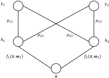
partition function is usually hard to compute. Fortunately, in the age distribution learning problem, the ultimate goal is to predict a distribution of description degree p(y♣x), we don't need to compute this normalization term and the suitable model is the conditional energy based model [Bengio et al., 2001; Schwenk and Gauvain, 2002]. Figure 1 shows a simple example of the energy based model. The formula of conditional probability mass function in Conditional Energy Label Distribution Learning (CE-LDL) model is given as:
where x is the input feature, y is the age index vector and h is the binary latent vector. The energy function of this model is set as:
The parameter set ✓ is ¶bj↪ ujr↪!r♣j 2 ¶1↪ 2↪ ▷▷▷↪ l♦↪ r 2 ¶1↪ 2▷▷▷↪ R♦♦. Here l is the number of ages and R is the number of latent variables. The number of feature extractors R, which is also the number of latent variables, is specified by users. Different forms of fr(x; !r) can be used in this model, e.g., linear form, quadratic form and sigmoid form.
By Bayesian rule, we can get:
Note that from Equation (5) to (6), we use the property of label index vector that only one element of this vector is 1, and the others are all 0. From Equation (7) to (8): we first expand the sums in Equation (7). Considering all hr are binary, we can then get Equation (8). The terms when hr = 0 become the 1 in the brackets. In the Equation (8), exp(bj) is the bias of the j th description degree, exp(fr(x; !r) + ujr) can be treated as the rth feature extractor. And ujr controls the effect of the rth feature extractor to j th description degree.
The rth feature extractor exp(fr(x; !r) +ujr) will return approximately 0 if this feature extractor does not fit the input feature x well. That means fr(x; !r) + ujr will get a very small value, which is far smaller than 0, then exp(fr(x; !r)+ ujr) will return approximately 0. Otherwise it will return a value which is larger than 1. For R feature extractors, this '0 or larger than 1' characteristic enables the model to learn exponential kinds of the input configurations, so CE-LDL can learn distributed representations.
3.2 The Comparsion of CE-LDL with some existent LDL methods
In [Geng et al., 2013], IIS-LDL was proposed to solve age distribution learning and then BFGS-LDL [Geng, 2016] was developed to accelerate the optimization process. Both of them are based on maximum entropy model and the p(yj = 1♣x) is defined as:
where !j is the parameter which need to be learned. From the perspective of energy based model, Equation (9) represents a two-layer energy based model. Compared with IIS-LDL and BFGS-LDL, the added hidden layer and the specially designed energy function can help CE-LDL extract more information from the complex features. Thus, the expressive ability of CE-LDL is stronger than IIS-LDL and BFGS-LDL.
The p(yj = 1♣x) used in CPNN-LDL [Geng et al., 2013] is:
where !j and βr are the parameters which need to be learned. CPNN-LDL can be treated as a three-layer model and it can indeed extract more information from input features than IISLDL and BFGS-LDL. However, compared with CE-LDL, it can hardly learn distributed representations. In CPNN-LDL, whether the feature extractor βr exp(fr(x↪ yj;!r)) fit the feature or not, it will return a value which will affect the model. When the training images are regular, the performance of CPNN-LDL is good. However, when the training images are not regular, the unfitted feature will return a value which will disturb the model. And thus, the performance of CPNN-LDL on some irregular image datasets will decline. In CE-LDL, the '0 or larger than 1' character enables the model to filter these unfitted features. So, even the training images are irregular, the performance of CE-LDL will not decline so much.
4 Sparsity Conditional Energy Label Distribution Learning model
Without the sparsity constraint, our model tends to learn distributed, non-sparse representations. And based on results from other methods [Olshausen and others, 1996; Lee et al., 2006; Bell and Sejnowski, 1997; Osindero et al., 2006; Poultney et al., 2006], sparseness enables the model to form Gabor-like filters, which is helpful in image analysis. Thus, the suitable sparsity constraints should be added. In order to illuminate how the sparsity constraints work, we first explain the role of binary latent vector h.
From Equation (2) and Equation (4) we can get:
Since the conditional probability p(yj = 1♣x↪ h) is proportion to p(x↪ yj = 1↪ h), then the conditional probability is also proportion to the products of a series of exponential functions (which are also the feature extractors as discussed in Section 3.1) exp(hr(fr(x;!r) + ujr)) and a bias term exp(bj). When binary latent variable hr is 1, the rth feature extractor can contribute to the conditional probability. Otherwise, the rth feature extractor returns 1 when hr is 0, that is to say, the rth feature extractor makes no contribution to the conditional probability. So hr can be understood as the trigger which controls the switch status of rth feature extractor.
In CE-LDL model, we can learn underlying factors which are informative to the task of age estimation, and in the sparsity amelioration one we want these factors to be more 'exclusive'. That is to say, we hope only a few feature extractors work (more feature extractor triggers hr should be 'off' status) given a feature x. Then the sparsity constraint term is given as follows:
The p(hr♣x↪ yj = 1) can be computed by using Bayesian rule and the result is given as follows:
For a given input feature x(i) , we know the description degree djx(i) of each label j. So the weighted average is used in Equation (12). Then the total objective function is the sum of Equation (1) and Equation (12) and we hope to find a ✓ to maximize such objective. That is:
where the λ controls the importance between the KL divergence with the sparsity constraints.
Batch stochastic gradient descent is used to solve Equation (15) and the derivatives of parameters of ln[p(yj = 1♣x)] are given as follows:
where the 1(j=k) is the indicator function which returns 1 when j = k and 0 otherwise. Derivatives of parameters of p(hr = 0♣x↪ yj = 1) are given as follows:
The learning algorithm is given in the Algorithm 1. After learning the parameters, given a new feature x⇤ , the predicted distribution p⇤ is computed by Equation (8) and the predicted age a⇤ is determined by a⇤ = argmaxa p⇤ (ya = 1♣x⇤ ).
Algorithm 1 Learning algorithm of SCE-LDL
Input:
The training set S.
Output:
The parameter set ✓.
- 1: Initialize the model parameter set ✓.
- 2: t = 0.
where tmax is the number of maximum iteration and ↵ is the learning rate. The derivatives of different parameters can be got by taking Equations (16)- (20) into Equation (15).
5 Experiments and analyses
5.1 Datasets used in the experiments
Two datasets are used in our experiments: MORPH [Ricanek Jr and Tesafaye, 2006] and the dataset provided by ChaLearn [Escalera et al., 2015]. There are totally 55,132 face images in the MORPH. The ages of the face images range from 16 to 77 with a median age of 33. The faces are from different races, among which the African faces account for about 77%, the European faces account for about 19%, and the remaining 4% includes Hispanic, Asian, Indian and other races. According to the chronological age of each face image, an age distribution is generated using the Gaussian distribution as follows:
where the a is the chronological age of the face image x and the σ is the standard deviation which is set as 1 here.
The second dataset used in the experiment is the ChaLearn dataset. There are totally 3,615 human images can be utilized in this dataset: 2,479 in the training set and 1,136 in the validation set. The images in this dataset are figure photos taken under wild condition. In order to get frontal face images from these human images, we pre-process these images by three steps. First, we employ DPMmodel [Mathias et al., 2014] to detect the main facial region of each image. Then the detected face is fed into a public available facial point detector software [Sun et al., 2013] to get the corresponding five facial key points including the left/right eye centers, nose tip and left/right mouth corners. Finally, based on these facial points, we utilize face alignment for these facial images.
In the ChaLearn dataset, the age of each image is labeled by multiple individuals as apparent age rather than its chrono-
| Methods | CE-LDL | SCE-LDL | BFGS-LDL | CPNN-LDL | OHR | KPLS |
| MORPH | 4▷146◦0▷080 | 3▷858◦0▷090 | 4▷872◦0▷055 | 4▷705◦0▷159 | 7▷085◦0▷009 | 4▷442◦0▷084 |
| ChaLearn | 6▷708 | 6▷432 | 7▷424 | 12▷979 | 7▷578 | 6▷841 |
m
m
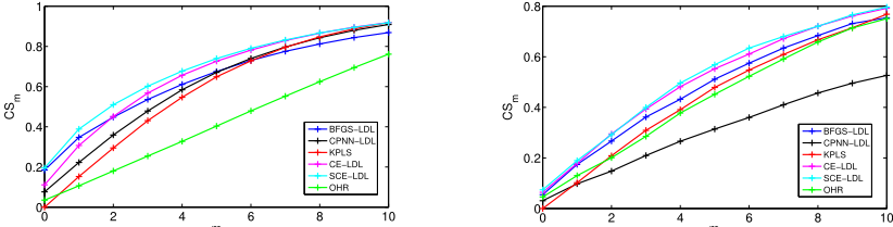
(a) CS of all the algorithms at the error levels 0-10 on the MORPH dataset. (b) CS of all the algorithms at the error levels 0-10 on the ChaLearn dataset.
Figure 2: The CS on MORPH and the CS on ChaLearn.
logical age. For each image, its mean age and the corresponding standard deviation are given. And in this dataset, these mean ages and standard deviations are used to generate the corresponding Gaussian distribution by Equation (21).
The features used for both datasets are Biologically Inspired Features (BIF) [Guo et al., 2009]. By simulating the primate visual system, BIF has shown good performance in facial age estimation [Guo et al., 2009]. In the MORPH dataset, the dimension of the BIF vectors is further reduced to 200 by using Marginal Fisher Analysis (MFA) [Yan et al., 2007]. In the ChaLearn dataset, only 2,479 images can be used to train our model, so we do not reduce the dimension of the extracted features. The 7,152 dimensional features are used in the ChaLearn dataset. In both datasets, the BIF features are normalized that the mean of each dimension is 0 and the variance of each dimension is 1.
5.2 Performance measurement
Two kinds of performance measurements are used in our experiments. The first one is Mean Absolute Error (MAE), i.e., the average absolute difference between the predicted age and the labeled age. The second one is cumulative score (CS), which is represented as follows:
where N is the total number of test images, Nm represents the number of probe facial images whose absolute error between the estimated age and the ground truth age is not greater than m years.
5.3 Experiment details
Three kinds of fr(x;!r) are attempted in our experiments: linear function, quadratic function and Sigmoid function. Similar results are got by using these three kinds of functions, while linear function have a quicker training speed. So the results of SCE-LDL reported in this section are computed by using linear function:
Some parameters used in the experiments are set as follows: the number of maximum iteration tmax is 30 and the learning rate ↵ is 0▷1. Some existing algorithms specially designed for facial age estimation are compared as the baseline methods, which include CPNN-LDL [Geng et al., 2013], BFGS-LDL [Geng, 2016], OHRank [Chang et al., 2011] and KPLS [Guo and Mu, 2011]. The reason of choosing these methods is that they almost get the best performance compared with some earlier age estimation methods.
And also note that we do not compare our methods with the results of competition which is held by ChaLearn because all the top-rank methods of that competition are based on deep learning [Escalera et al., 2015]. And in the competition, these deep learning methods collected a huge number of additional facial images to train their deep architectures. But we only use the given 2,479 facial images to train our model.
5.4 Experiment results and analyses
In the first experiment, MORPH dataset is randomly split into 10 chunks. Each time, 1 chunk is used as the testing set and the rest 9 chunks are used as the training set. This procedure is repeated 10 folds and the mean value and standard deviation of each evaluation measure is computed. The number of hidden units R is set as 150 and the λ is set as 0▷005. The first row of Table 1 reports the MAE of all the compared methods on the MORPH dataset. Figure 2a shows the CS of all the compared methods at the Error Levels 0-10 on the MORPH dataset.
In the second experiment, we use the images in training set provided by ChaLearn to train our model. And the validation set provided by ChaLearn is used as the test set in our experiment. The number of hidden units R is set as 150 and the λ
| R | 50 | 75 | 100 | 125 | 150 | 175 |
| MORPH | 3▷963◦0▷076 | 3▷905◦0▷077 | 3▷868◦0▷090 | 3▷874◦0▷090 | 3▷858◦0▷090 | 3▷842◦0▷101 |
|---|---|---|---|---|---|---|
| ChaLearn | 6▷774 | 6▷607 | 6▷577 | 6▷619 | 6▷432 | 6▷473 |
| λ | 0 | 0.001 | 0.005 | 0.01 | 0.05 |
|---|---|---|---|---|---|
| MORPH | 4▷146◦0▷118 | 3▷936◦0▷127 | 3▷858◦0▷090 | 3▷883◦0▷089 | 3▷960◦0▷080 |
| ChaLearn | 6▷708 | 6▷666 | 6▷432 | 6▷768 | 6▷784 |
is set as 0▷005. The second row of Table 1 reports the MAE of all the compared algorithms on the ChaLearn dataset. Figure 2b shows the CS of all the compared methods at the Error Levels 0-10 on the ChaLearn dataset.
As can be seen in the Table 1, the performances of CELDL and SCE-LDL are significantly better than other age estimation algorithms. And after incorporating the sparsity constraints, the performance improves. Compared with the MAEs of all methods on the MORPH dataset, the MAEs computed on ChaLearn dataset are generally worse. This is because that, in the MORPH dataset, the images are frontal faces taken indoor with similar lighting, while the images of another one, ChaLearn, are figure photos taken under wild condition. Though we have pre-processed these photos, the pre-processed facial images in ChaLearn are not as regular as the facial images in MORPH.
From the Figure 2a, we can see that, in the MORPH dataset, different methods (except OHR) get similar CS values at high error levels. But at lower error levels, SCE-LDL obviously owns the highest CS. This also means that SCELDL is more accurate than other age estimation methods on the MORPH dataset.
In the ChaLearn dataset, only 2,479 images are used to train each model. And as discussed in Section 1, compared with single label methods, one major advantage of LDL methods is that LDL methods can use a dataset more sufficiently. Thus, the performances of BFGS-LDL, CE-LDL and SCELDL are better than KPLS and OHR, as shown in Figure 2b.
As discussed in Section 3.2, since SCE-LDL can learn a model with stronger expressiveness, the performance of SCE-LDL is generally better than BFGS-LDL and CPNNLDL. And although CPNN-LDL can extract more information from features than BFGS-LDL, some parts of this information will disturb the model. So when the number of training images is large and the training images are regular, such as MORPH dataset, the performance of CPNN-LDL is good. But when the number of training images becomes fewer and when the images are took under wild condition, such as ChaLearn dataset, the performance of CPNN-LDL declines. Since SCE-LDL can learn distributed representations, then the unfitted features will be filtered, the performance of SCE-LDL will not decrease so much compared with CPNN-LDL.
Table 2 shows the MAE of SCE-LDL computed by using different R, and here the λ is set as 0▷005. This table shows that the predicted result is not very sensitive to the choice of R. For both datasets, even in the worst case (when R is 50), the MAEs of SCE-LDL on both datasets are lower than the other methods. Table 3 shows the MAE of SCELDL computed by using different λ, and here the R is set as 150. The choice of λ is important because it controls the balance between KL divergence and sparsity constraints. On the one hand, if λ is too small, the SCE-LDL will trend to learn non-sparse representations, then SCE-LDL degenerates to CE-LDL. On the another hand, if λ is too big, in the Equation (15), the effect of KL divergence will be weakened, then the predicted distribution will be less similar with the real distribution. But if λ is chosen from a suitable range, as shown in Table 3, the performance will not have huge fluctuations.
6 Conclusion
In this paper, SCE-LDL is proposed to estimate ages from face images. In SCE-LDL, we assign a Gaussian distribution to each face image and use these age distributions as the training targets. And energy function is used to define the age distribution. By assigning a suitable type of energy function to the model, SCE-LDL can learn distributed representations while other LDL methods can hardly do. Thus, SCE-LDL have the ability to learn a model with stronger expressiveness compared with IIS-LDL, BFGS-LDL and CPNN-LDL. In order to help the model learn distributed sparse representations, sparsity constraints are also incorporated to improve the performance of the model. At last, the experiment results of two different datasets show that our proposed SCE-LDL can get the best performances compared with the baseline algorithms.
Acknowledgement
This research was supported by the National Science Foundation of China (61273300, 61232007,61528302), the Jiangsu Natural Science Funds for Distinguished Young Scholar (BK20140022), and the Collaborative Innovation Center of Wireless Communications Technology.
@inproceedings{ijcai2016p322,
  title     = {Sparsity Conditional Energy Label Distribution Learning for Age Estimation},
  author    = {Yang, Xu and Geng, Xin and Zhou, Deyu},
  booktitle = {Proceedings of the Twenty-Fifth International Joint Conference on
               Artificial Intelligence, {IJCAI-16}},
  publisher = {AAAI Press / International Joint Conferences on Artificial Intelligence},
  editor    = {Subbarao Kambhampati},
  pages     = {2259--2264},
  year      = {2016},
  month     = {7},
  url       = {https://ijcai.org/proceedings/2016/322},
}
TY - CPAPER TI - Sparsity Conditional Energy Label Distribution Learning for Age Estimation AU - Yang, Xu AU - Geng, Xin AU - Zhou, Deyu T2 - Proceedings of the Twenty-Fifth International Joint Conference on Artificial Intelligence, IJCAI-16 PB - AAAI Press / International Joint Conferences on Artificial Intelligence PY - 2016 SP - 2259 EP - 2264 UR - https://ijcai.org/proceedings/2016/322 ER -Copied
Machine-readable versions of this paper, for tools and AI agents:





