Frequent Direction Algorithms for Approximate Matrix Multiplication with Applications in CCA

1 Introduction

Modern large data sets are often expressed as large matrices. For example, in the bag-of-words model, each row of the matrix corresponds to one document; in image analysis, feature values are represented by a matrix whose rows correspond to images. Therefore, many computational problems on such data are reduced to standard matrix operations including matrix multiplication, `2-regression, and low-rank matrix approximation.

Some data are huge in size and often generated sequentially, e.g., computer network traffic and sensor data. Thus, it is important to handle them in a streaming fashion. A streaming algorithm only makes a single pass over the data and uses a small amount of memory. The limited space constraint is critical when the full data set cannot fit in memory or even disk. Typically, there is a trade-off between the amount of space required and the performance of the algorithm.

Approximate matrix multiplication gains significant increases in popularity as the data sets becoming larger and larger. It is an important approach to fast matrix multiplication. Moreover, it can be used in information retrieval [Eriksson-Bique et al., 2011], image processing [Madrid et al., 2012], large scale k-means clustering [Cohen et al., 2015], and approximate leverage scores [Drineas et al., 2012]. The best approximation to the product can be achieved by truncated SVD under any unitarily invariant norms. Although SVD methods are polynomial, they are computation intense when performed exactly.

There are two main approaches for approximate matrix multiplication. The first approach is referred as random selection since it randomly picks rows, columns, or individual entries of the matrices. There are two kinds of sampling methods: uniform sampling and non-uniform sampling. Most studies focus on the latter which obtains more generality. One important non-uniform sampling method is called importance sampling which works with probability proportional to the row's squared Euclidean length [Drineas and Kannan, 2001; Drineas et al., 2006; Eriksson-Bique et al., 2011]. Madrid et al. (2012) compared different sampling strategies on illconditioned matrices empirically. Pagh (2013) focused on sparse matrices.

The second approach is referred as random projection or "sketching." Many studies are based on the JohnsonLindenstrauss (JL) Lemma [Dasgupta and Gupta, 2003]. For example, Sarlos (2006) achieved a Frobenius norm error guarantee using the JL transform. Clarkson and Woodruff (2009) further refined the results, and showed that their space usage is nearly optimal in a streaming setting. Kane and Nelson (2014) gained more speed up by introducing a sparse JL transform. Clarkson and Woodruff (2013) came up with a very sparse subspace embedding matrix with modifications by Nelson and Nguyˆen (2013). Their work reduced time complexity to O(nnz(A) + nnz(B)). However, random projection may fail with relatively high probability when sketch size is small.

Besides these two main kinds, there are also some other methods. For example, Cohen et al. (2015) proved that using subspace embedding achieves optimal approximate matrix multiplication in terms of stable rank. Bhojanapalli et al. (2015) proposed a new method which utilizes sampling and alternating minimization to directly compute a low-rank approximation of matrix product. However, those methods can not be implemented in a streaming way.

In this paper we investigate the streaming memory-limited matrix multiplication problem. Our work is inspired by a recently proposed matrix sketching algorithm called the Frequent-Directions (FD) [Liberty, 2013] which is easy to implement and deterministic. We propose a new method for approximate matrix multiplication (AMM) that we call FDAMM. To our best knowledge, our method is the first deterministic approach to approximate matrix multiplication. An error bound in terms of spectral norm is given, and experimental results demonstrate its effectiveness and efficiency.

We also apply our approach to computing Canonical Correlation Analysis (CCA) of two matrices in a streaming way. CCA is a fundamental statistical tool to capture the relationship between two multidimensional variables [Hotelling, 1936]. It is analogous to Principal Component Analysis (PCA). But instead of analyzing a single matrix, it aims to analyze the relation between a pair of datasets. It has found its usage in a wide range of applications, e.g., dimensionality reduction [McWilliams et al., 2013], clustering [Chaudhuri et al., 2009], and speech recognition [Wang et al., 2015].

The remainder of the paper is organized as follows. We first define the notation used in this paper and introduce the background of CCA and FD algorithm. Then we describe our proposed FD-AMM method and provide theoretical analysis in section 3. Finally, we provide empirical comparisons with three most used AMM algorithms to demonstrate the superiority of FD-AMM.

2 Notation and Preliminaries

In this section we give the notation and preliminaries which will be used in this paper. We use i : j to denote the integer set ¶i↪ ▷ ▷ ▷ ↪ j♦, and define [n] = 1 : n. Let In be the n ⇥ n identity matrix, and 0 be the matrix of zeros with appropriate size. We are given an n ⇥ m matrix A = [a1; a2; ▷ ▷ ▷ ; an] where ai 2 R1⇥m is the i-th row of A. Typically the matrix is assumed to be thin so n ≥ m. When matrices A and B have the same number of rows, we use [A B] to denote the matrix obtained by concatenating the columns of B next to the columns of A. Two vectors x and y are orthogonal is denoted by x ? y.

The singular value decomposition of A 2 Rm⇥n , written svd(A), produces three matrices ¶U↪⌃↪V♦ so that A = U⌃VT where U 2 Rn⇥n and V 2 Rm⇥n satisfy UT U = UUT = VT V = In, and ⌃ is an n ⇥ n diagonal matrix with singular values σ1 ≥ σ2 ≥ · · · ≥ σn ≥ 0. Let r be the rank of A. Assume eU and eV consist of the first r columns of U and V respectively, and e⌃ = diag(σ1↪ σ2↪ ▷ ▷ ▷ ↪ σr), then eUe⌃eV = A is the condensed SVD of A. The SVD of an n ⇥ m matrix costs time O(mn min¶n↪ m♦).

The squared Frobenius norm of the matrix A is defined as kAk2F = Pni=1 kaik2 where kaik is the Euclidean norm of row ai. The spectral norm is kAk2 = maxx:kxk=1 kAxk.

Then we formally introduce the background of CCA. There are several equivalent ways to define the canonical correlations of a pair of matrices [Golub and Zha, 1995]. Here we use the linear algebraic formulation described in Definition 2.1, which captures the very essence of the procedure, pursuing the directions of maximal correlations between two data matrices.

Definition 2.1. [Avron et al., 2014] LetA 2 Rn⇥m1 andB 2 Rn⇥m2 , and assume that p = rank(A) ≥ rank(B) = q. The canonical correlations ⇡1(A↪B) ≥ ⇡2(A↪B) ≥ · · · ≥ ⇡q(A↪B) of the matrix pencil (A,B) are defined recursively by the following formula:

where

• ÷ i = 1↪ ▷ ▷ ▷ ↪ q,
• ÷ Ai = ¶x : Ax 6= 0↪ Ax ? ¶Ax1↪ ▷ ▷ ▷ ↪ Axi-1♦♦,
• ÷ ⇡(u↪ v) = ♣uT v♣◁(kukkvk),
• ÷ Bi = ¶y : By 6= 0↪ By ? ¶By1↪ ▷ ▷ ▷ ↪ Byi-1♦♦.

The n-dimensional unit vectors

are called canonical vectors.

There are quite a few methods to compute the canonical correlations [Golub and Zha, 1995]. For example, Bj¨orck and Golub (1973) proposed an algorithm based on Theorem 1, which needs exactly QR decomposition of original matrices A and B.

Theorem 2 can be proved directly by the definition of CCA [Lu and Foster, 2014]. The approach based on Theorem 2 needs matrix multiplication AT A and BT B with O(n(m21 + m22 )) computational complexity and matrix decomposition to compute S- 12 a and S- 12 b with O(m31 + m32 ) computational complexity. As a result, both two methods require O(n(m21 + m22 )) time and O(n(m1 + m2)) space. These classical methods are feasible and accurate when the data matrices are small but they can be slow and unstable for large-scale datasets.

Theorem 1. [Bj¨orck and Golub, 1973] Assume that the columns of Q 2 Rn⇥p and W 2 Rn⇥q form an orthonormal basis for the range of A and B, respectively. Let QT W = eUe⌃eVT be its condensed SVD. The diagonal elements of e⌃ are the canonical correlations of (A↪B)▷ The canonical vectors are given by the first q columns of Q eU for A and of WeV for B.

Theorem2. [Lu and Foster, 2014] Let Sa =AT A◁n, Sb = BT B◁n and Sab = AT B◁n. Let S- 12 a SabS- 12 b = eUe⌃eVT be its condensed SVD. Then the diagonal elements of e⌃ are the canonical correlations of (A↪B). The canonical vectors are given by the first q columns of S- 12 a eU forAand of S- 12 b eV for B.

3 Methodology

In this section, we first review the Frequent Directions algorithm. Then we present the main contribution of the paper: the FD-AMM algorithm. Specifically, given an n⇥m1 matrix A and an n ⇥m2 matrix B, FD-AMM computes an approximation X to the product AT B so that X ⇡ AT B. Moreover, the algorithm is based on a streaming setting which only requires one pass over the input. Finally, we give a new way to compute the CCA of two matrices also in a streaming fashion which is based on FD-AMM.

We describe the procedure of FD algorithm [Liberty, 2013; Ghashami and Phillips, 2014] in Algorithm 1. FD computes a sketch of a given matrix. Specifically, it keeps an ` ⇥ d (`  n) sketch matrix H that is updated every time a new row from the n ⇥ d input matrix G is added. For any unit vector x 2 Rd , it has

The algorithm maintains an invariant that the last row of the sketch H is always all-zero valued. During the execution of the algorithm, rows from G simply replace the all-zero valued row in H. Then, the last row is nullified by a twostage process. First, we rotate the sketch matrix by SVD so that its rows are in descending order of significance.Then, we "shrink" all the rows so that at least one of them becomes zero.

Algorithm 1 Frequent Directions (FD)

Input: `↪G 2 Rn⇥d H = 0`⇥d for i 2 1↪ ▷ ▷ ▷ ↪ n do h` = gi [Z↪ S↪ Y] =svd(H) M(i) = SYT [only for notation] δi = s2` [the `th entry of S, squared] S0 = pS2 - δiI` H(i) = S0YT end for return H=H(n)

The computational cost of each iteration comes from the SVD of an ` ⇥ d matrix, which is O(d`2 ) when ` < d. The total time complexity of FD algorithm is therefore bounded by O(nd`2 ).

3.1 FD-AMM

Algorithm 2 FD-AMM

Input: `↪A 2 Rn⇥m1 ↪B 2 Rn⇥m2 G = [A B] H = FD(`↪ G) C = H[`]↪1:m1 D = H[`]↪m1+1:m1+m2 return X=CT D

We presents the proposed method FD-AMM in Algorithm 2. It is built upon the FD algorithm, but it focuses on the approximate product of two given matrices. We provide the theoretical guarantee of FD-AMM algorithm in Theorem 3. The proof of the theorem is presented in the appendix.

Theorem 3. If X is the result of applying the FD-AMM algorithm to matrices A, B, and sketch size `, then

Liberty (2013) observed that the time complexity of FD algorithm can be reduced to O(nd`) at the expense of more space. More specifically, increasing ` by a constant c > 1 and then processing every `(c - 1) elements in a batch setting (each round results in a c` rows matrix H) can reduce the overall time to O( c2 c-1 nd`). This trick can be applied to our algorithm. Let `new = 2`old then the time complexity becomes O(2nm`new). Thus our FD-AMM algorithm can run in O(nm`), where m = m1 + m2.

Using FD-AMM for approximate matrix multiplication has several advantages. First, it is easy to implement. Second, the error bound given by Theorem 3 is stronger than existing state-of-art algorithms with the same sketch size `. It is worth pointing out that both sampling and random projection based algorithms' error bounds are proportional to 1◁p`. Third, our algorithm is deterministic. Hence it is more stable than other random algorithms.

3.2 Streaming CCA

Based on the FD-AMM algorithm, we come up with a new way to calculate the canonical correlations of two matrices. The new method is inspired by a special case of the FDAMM algorithm. When ` ≥ 2m, we have δi = 0 for all i = 1↪ ▷ ▷ ▷ ↪ n, which makes the "shrink" step does nothing at all thus can be omitted. As a result we have H(i) = M(i) and H(i-1) T H(i-1) = H(i) T H(i) . Therefore, the total error incurred by FD-AMM is still zero. Corollary 4 gives the formal observation. The proof of Corollary 4 is similar to that of Theorem 3.

Corollary 4. In Theorem 3, when ` ≥ 2m, we will have δi = 0 for all i = 1↪ ▷ ▷ ▷ ↪ n. Thus the total error incurred by the FD-AMM algorithm is zero. More specifically,

With the same reason, we have AT A = CT C and BT B = DT D in this case.

The streaming nature of our FD-AMM algorithm helps especially when the matrices are too large to fit in memory. To be specific, when given a pair of matrices (A↪B), we transform the pair to a new pair (C↪D) that has much fewer rows, and then compute the canonical correlations of the new pair exactly, e.g., using the Bj¨orck and Golub algorithm. We present the detailed procedure in Algorithm 3. Theoretical analysis is given in Theorem 5.

Theorem 5. If the two matrices A and B are tall-and-thin, that is, n ≫ m1, then Algorithm 3 computes the exact canonical correlations of (A↪B). That is,

for i = 1↪ ▷ ▷ ▷ ↪ q. And the canonical vectors returned by Algorithm 3 are the same as the results computed by the Bj¨orck and Golub algorithm.

Combining Theorem 2 and Corollary 4 can get Theorem 5 directly. Algorithm 3 has a time complexity of O(nm2 ) and space complexity of O(m2 ), while the Bj¨orck and Golub algorithm needs O(nm) space.

Algorithm 3 Streaming CCA

Input: A 2 Rn⇥m1 of rank p and B 2 Rn⇥m2 of rank q (m1 ≥ m2, p ≥ q). m = m1 + m2, ` = 2m. G = [A B], H = 0`⇥m. for i 2 1↪ ▷ ▷ ▷ ↪ n do Insert gi into a zero valued row of H if H has no zero valued rows then [Z↪ S↪ Y] =svd(H) H = SYT end if end for return H= [CD]

Compute and return the canonical correlations and the canonical vectors of (C↪D) (using classical algorithm).

4 Experiments

We compare FD-AMM with baselines. The first one is the brute force approach. The other three are common algorithms that are used in practice: sampling, random projection, and sparse random projection. All methods receive the rows of an n⇥m1 matrix A and an n⇥m2 matrix B one by one during the experiments. The brute force method outputs the product directly, while other methods first compute smaller matrices C and D for A and B respectively, then compute CT D.

Brute Force (BF): The brute force approach produces the exact result of AT B. It explicitly computes the matrix AT B = Pni aTi bi by aggregating the outer products of the rows of A and B. The update time of Brute Forces is O(m1m2) and its space complexity is O(m1m2).

Sampling: Let pi = kaikkbik◁S be a probability distribution over [n] where S = Pni=1 kaikkbik. We form an ` ⇥ m1 matrix C and an ` ⇥ m2 matrix D by taking ` i.i.d. (row indices) samples with the pi. Since the value of S is not known a priori, we use ` independent reservoir samplers to implement the streaming algorithm. Therefore, the update for each row requires O(m1 +m2) time and O(`(m1 + m2)) space. The reader can refer to [Drineas et al., 2006; Eriksson-Bique et al., 2011] for a theoretical analysis of this algorithm.

Random projection (RP): The matrices C and D have the form of RA and RB respectively, where R is an ` ⇥ n matrix and Rij 2 ¶-1◁p`↪ 1◁p`♦ uniformly. This is easily computed in a streaming fashion, while requiring at most O(`(m1 + m2)) space and O(`(m1 + m2)) time per row. For proofs of effectiveness and usage see [Clarkson and Woodruff, 2009; Cohen et al., 2015].

Sparse Random Projection (SRP): Clarkson and Woodruff (2013) proposed a very sparse projection matrix S, which has exactly 1 non-zero element per column. The element can be -1 or +1 uniformly. To implement this algorithm in streaming manner, matrices C and D are generated by adding or subtracting the rows of A and B randomly. More specifically, C and D are initialized to be ` ⇥m1 and ` ⇥m2 all zeros matrices. When processing rows of A and B, we perform ch(i) ch(i) + s(i)ai and dh(i) dh(i) + s(i)bi, where h: [n] ! [`] and s: [n] ! ¶-1↪ 1♦ are perfect hash functions.

4.1 Approximate MatrixMultiplication

In this section, both A and B are random matrices. Each entry of A and of B is independent and uniformly distributed on [0↪ 1]. For random algorithms, we execute 50 times for each sketch size and report the corresponding means and variances. The experiments are conducted in Matlab and run on a PC with Intel Core i5 CPU,4GB RAM, and Windows 7 64bit system. The Matlab is set in single thread mode when evaluating time. The performance is measured in terms of accuracy, stability, and speed.

Accuracy

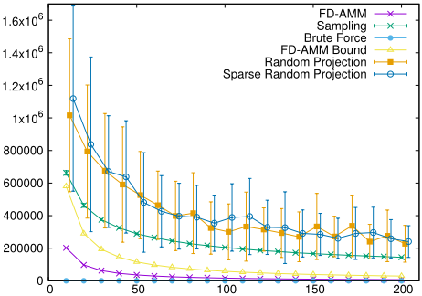
Accuracy is calculated by kAT B - CT Dk2. In the first experiment, the product of two moderately sized matrices (10000 ⇥ 1000 and 10000 ⇥ 2000) is approximated by the algorithms described above. Figure 1 shows the average accuracy with standard deviation over 50 trails when ` is set to different values. We shift the plots denoted by "Random Projection" and "Sparse Random Projection" a little bit right so they would not overlap with each other. Our results are similar with [Liberty, 2013]. Some key findings are listed below. First, the plot denoted by "FD-AMM Bound" is the theoretical worst case guaranteed by FD-AMM. It illustrates that our algorithm performs significantly better than expected by its worst case analysis. Second, the "FD-AMMBound" is lower than the random methods all the time. It suggests that even the guaranteed worst case is lower than those of competing algorithms. Third, the three random algorithms perform equally well when considering the best results in 50 trials. The sampling method achieves better average accuracy compared to random projection and sparse random projection.

Stability

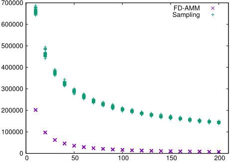
Now we compare the stability of different algorithms. As mentioned earlier, FD-AMM is a deterministic method which returns the same output every time, while the other three methods are random algorithms. As Figure 1 shown, the accuracy achieved by the random projection and sparse random projection algorithms fluctuates widely between different trials, while the sampling method is more stable. Also, we can find the better stability can be achieved with large sketch size `, which is consistent with our intuition. Furthermore, we plot all the computation results of the sampling and FD-AMM methods in Figure 2. Even though the row sampling method yields a better approximation to the product compared to random projection and sparse random projection, it is still not deterministic.

Speed

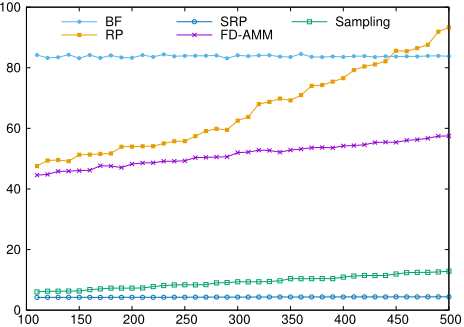
The running time of our algorithm is between that of random projection and sampling. In Figure 3, the running time of different AMM algorithms are plotted as a function of their sketch sizes. We have some interesting observations here. First, the larger the sketch size, the longer the running time. However, the Brute Force method computes AT B directly, so its running time is independent of `. Second, the Sparse Random Projection method is fast and independent of `, but it's only slightly better than the Sampling method. Third, although FD-AMM shares the same theoretical time complexity (O(n`(m1 +m2))) with random projection, our method scales better.

4.2 Streaming CCA on Real-life Data

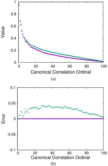
In this section, we test our streaming CCA algorithm on the annotated video dataset from the Mediamill Challenge [Snoek et al., 2006]. There are 43907 images in total. Each image is a representative key frame of a video shot with 120 features and the whole set is annotated with 101 labels. We perform CCA to analyze the correlation structure between the features and labels. Figure 4(a) shows the canonical correlations and 4(b) shows the relative error. From the Figure 4(a), we can see that a few high correlations exist between the features and labels, with strong decay afterward. Figure 4(b) shows that the results of Streaming CCA are exactly the same as the results computed by the traditional method [Bj¨orck and Golub, 1973]. We compare the running time with the traditional method and the approximation algorithm in [Avron et al., 2014]. It turns out that the Streaming CCA (taking 4.69 sec) is a little faster than traditional method (taking 5.93 sec) and slower than the approximation method (taking 2.51 sec).

5 Conclusions

In this paper, we have proposed a deterministic algorithm to compute the approximation of matrix product in a streaming way and provided theoretical analysis for the approximation performance. The experiments have shown that our algorithm is much more accurate than the other three random methods with an acceptable speed. We have applied our approach to computing CCA, giving rise to a fast streaming method. The experiments on real-world dataset have also validated the effectiveness of the method.

Acknowledgments

This work has been supported by the National Natural Science Foundation of China (No. 61572017), Natural Science Foundation of Shanghai City (No. 15ZR1424200), and Microsoft Research Asia Collaborative Research Award.

Appendix: Proof of Theorem 3

Let H(i) = [C(i) D(i) ] and M(i) = [P(i) Q(i) ]. Let Y = [Y1;Y2], where Y1 is the first m1 rows of Y, and Y2 is the remaining m2 rows of Y. Let ai and bi denote the i-th row of A and B. In what follows, we denote by δi, P(i) , Q(i) , C(i) , D(i) the values of δ, P, Q, C and D respectively after the main loop in the algorithm has been executed i times. Let 4 = Pni=1 δi be the total mass we subtract from the stream during the algorithm. We start by proving three useful lemmas.

Lemma 6. (Corollary 3.1.3 of [Horn and Johnson, 2012]) Let A 2 Rn⇥m be given, and let Ar denote a submatrix of A obtained by deleting a total of r rows and/or columns from A. Then

Lemma 7. For any unit vector x1 2 Rm1 and x2 2 Rm2 , we have xT1 P(i) T Q(i)x2 - xT1 C(i) T D(i)x2  δi.

In the last inequality, we use Lemma 6.

Lemma 8. For any unit vector x1 2 Rm1 and x2 2 Rm2 , we have 0  xT1 AT Bx2 - xT1 CT Dx2  4.

Proof. Notice that for all 2  i  n, we have

By substituting this into inequality from Lemma 7, we get xT1 C(i-1) T D(i-1)x2 + xT1 aTi bix2  xT1 C(i) T D(i)x2 + δi Subtracting xT1 C(i-1) T D(i-1)x2 from both sides and summing over i reveals

To see the first inequality observe xT1 C(i-1) T D(i-1)x2 + xT1 aTi bix2 = xT1 P(i) T Q(i)x2 ≥ xT1 C(i) T D(i)x2 for all 1  i  n. Then we can expand

With Lemma 8, we are ready to prove the main theorem.

Theorem 3.

Using that kCk2F + kDk2F ≥ 0 we obtain 4  (kAk2F + kBk2F )◁`. Recall that for any unit vector x1 2 Rm1 and x2 2 Rm2 ,

kAT B-CT Dk2 = sup x1↪x2 ♣xT1 (AT B-CT D)x2♣▷ Combining Lemma 8, we get 0  kAT B - CT Dk2  4  (kAk2F + kBk2F )◁`▷