
Self-Adapted Multi-Task Clustering
Proceedings of the Twenty-Fifth International Joint Conference on Artificial Intelligence. Pages 2357-2362.
Abstract
Multi-task clustering improves the clustering performance of each task by transferring knowledge across related tasks. Most existing multi-task clustering methods are based on the ideal assumption that the tasks are completely related. However, in many real applications, the tasks are usually partially related, and brute-force transfer may cause negative effect which degrades the clustering performance.In this paper, we propose a self-adapted multi-task clustering (SAMTC) method which can automatically identify and transfer reusable instances among the tasks, thus avoiding negative transfer. SAMTC begins with an initialization by performing single-task clustering on each task, then executes the following three steps: first, it finds the reusable instances by measuring related clusters with Jensen-Shannon divergence between each pair of tasks, and obtains a pair of possibly related subtasks;second, it estimates the relatedness between each pair of subtasks with kernel mean matching;third, it constructs the similarity matrix for each task by exploiting useful information from the other tasks through instance transfer, and adopts spectral clustering to get the final clustering result. Experimental results on several real data sets show the superiority of the proposed algorithm over traditional single-task clustering methods and existing multitask clustering methods.
- [Al-Stouhi and Reddy, 2014] Samir Al-Stouhi and Chan- dan K. Reddy. Multi-task clustering using constrained symmetric non-negative matrix factorization. In SIAM, pages 785-793, 2014.
- [Chen and Cai, 2011] Xinlei Chen and Deng Cai. Large scale spectral clustering with landmark-based representa- tion. In AAAI, pages 313-318, 2011.
- [Gu and Zhou, 2009] Quanquan Gu and Jie Zhou. Learning the shared subspace for multi-task clustering and trans- ductive transfer classification. In ICDM, pages 159-168, 2009.
- [Gu et al., 2011] Quanquan Gu, Zhenhui Li, and Jiawei Han. Learning a kernel for multi-task clustering. In AAAI, pages 368-373, 2011.
- [Gupta et al., 2013] Sunil Kumar Gupta, Dinh Q. Phung, Brett Adams, and Svetha Venkatesh. Regularized nonneg- ative shared subspace learning. Data Min. Knowl. Discov., 26(1):57-97, 2013.
- [Huang et al., 2006] Jiayuan Huang, Alexander J. Smola, Arthur Gretton, Karsten M. Borgwardt, and Bernhard Schölkopf. Correcting sample selection bias by unlabeled data. In NIPS, pages 601-608, 2006.
- [Jarvis and Patrick, 1973] R. A. Jarvis and E. A. Patrick. Clustering using a similarity measure based on shared nearest neighbors. IEEE Trans. Comput., 22(11):1025- 1034, 1973.
- [Jiang et al., 2013] Bin Jiang, Jian Pei, Yufei Tao, and Xuemin Lin. Clustering uncertain data based on probabil- ity distribution similarity. IEEE Trans. Knowl. Data Eng., 25(4):751-763, 2013.
- [Kullback and Leibler, 1951] Solomon Kullback and Richard A. Leibler. On information and sufficiency. The Annals of Mathematical Statistics, 22(1):79-86, 1951.
- [Lin, 1991] Jianhua Lin. Divergence measures based on the shannon entropy. IEEE Trans. Inform. Theory, 37(1):145- 151, 1991.
- [Pan and Yang, 2010] Sinno Jialin Pan and Qiang Yang. A survey on transfer learning. IEEE Trans. Knowl. Data Eng., 22(10):1345-1359, 2010.
- [Shi and Malik, 2000] Jianbo Shi and Jitendra Malik. Nor- malized cuts and image segmentation. IEEE Trans. Pat- tern Anal. Mach. Intell., 22(8):888-905, 2000.
- [Silverman, 1986] Bernard W. Silverman. Density estima- tion for statistics and data analysis, volume 26. CRC press, Boca Raton, FL, USA, 1986.
- [Wen et al., 2015] Junfeng Wen, Russell Greiner, and Dale Schuurmans. Correcting covariate shift with the frank- wolfe algorithm. In IJCAI, pages 1010-1016, 2015.
- [Xie et al., 2012] Saining Xie, Hongtao Lu, and Yangcheng He. Multi-task co-clustering via nonnegative matrix fac- torization. In ICPR, pages 2954-2958, 2012.
- [Xu et al., 2003] Wei Xu, Xin Liu, and Yihong Gong. Doc- ument clustering based on non-negative matrix factoriza- tion. In SIGIR, pages 267-273, 2003.
- [Zhang and Zhang, 2010] Jianwen Zhang and Changshui Zhang. Multitask Bregman clustering. In AAAI, pages 655-660, 2010.
- [Zhang and Zhang, 2013] Xianchao Zhang and Xiaotong Zhang. Smart multi-task Bregman clustering and multi- task Kernel clustering. In AAAI, pages 1034-1040, 2013.
- [Zhang and Zhou, 2012] Zhihao Zhang and Jie Zhou. Multi- task clustering via domain adaptation. Pattern Recogni- tion, 45(1):465-473, 2012.
- [Zhang et al., 2015] Xianchao Zhang, Xiaotong Zhang, and Han Liu. Smart multitask bregman clustering and mul- titask kernel clustering. ACM Trans. Knowl. Disc. Data, 10(1):8, 2015.
- [Zhang, 2015] Xiao-Lei Zhang. Convex discriminative mul- titask clustering. IEEE Trans. Pattern Anal. Mach. Intell., 37(1):28-40, 2015.
References were extracted automatically from the PDF and may contain errors.
Full text extracted automatically from the PDF; figures, tables and equations may differ. The PDF is the version of record.
1 Introduction
Traditional clustering algorithms deal with a single clustering task on a single data set. However, the information in a single data set may be too limited to help reveal the correct cluster structure. Multi-task clustering improves the clustering performance of each task by transferring knowledge across related tasks. There are mainly two ways to transfer knowledge in multi-task clustering [Pan and Yang, 2010]: instance transfer reuses certain parts of the data from the other tasks for each task; feature representation transfer learns a common feature representation among the related tasks. Most existing multi-task clustering methods are based on the assumption that the tasks are completely related, i.e., the label spaces among the tasks are the same. However, in many real applications, the tasks are usually partially related, i.e., only parts of the label spaces among the tasks are the same. Transferring knowledge of instances not in the related label space may degrade the clustering performance, this is referred to as negative transfer [Pan and Yang, 2010]. For example, if we have two tasks to cluster web pages from two universities by institute, one university contains the web pages under the institutes of Mathematics, Engineering and Medicine, the other university contains the web pages under the institutes of Mathematics, Engineering and Business. Only the web pages under the institutes of Mathematics and Engineering are reusable for multi-task knowledge transfer, and transferring knowledge of the web pages under the institutes of Medicine and Business may cause negative effect.
Two kinds of multi-task clustering methods for partially related tasks based on some assumptions have been proposed: 1) MBC [Zhang and Zhang, 2010] and its improved versions S-MBC and S-MKC [Zhang and Zhang, 2013] update the clusters by learning the relationship between clusters of different tasks. However, they work for the case that the distributions of the tasks are the same or similar (most data points of the tasks are from the same distribution); 2) MTRC [Zhang, 2015] learns the task relatedness through Gaussian prior, but it is based on a strict assumption that all tasks have the same cluster number and the label marginal distribution in each task distributes evenly. In light of the limitations of the existing multi-task clustering methods, it is urgent to develop a more general multi-task clustering method for partially related tasks.
In this paper, we propose a self-adapted multi-task clustering (SAMTC) method which can automatically identify and transfer reusable instances among the tasks, thus avoiding negative transfer when the tasks are partially related. In the multi-task setting, each task can be seen as a target task, and the other tasks are source tasks. Based on the assumption that if the given tasks are related, there are certain parts of instances from the source tasks that can be reused for clustering each target task [Pan and Yang, 2010]. The intention of SAMTC is to identify such parts and transfer knowledge among them. SAMTC begins with an initialization by performing single-task clustering on each task, then executes the following three steps. 1) Reusable instances finding: it computes the distance of any two clusters between each pair of target task and source task with a common distribution measure Jensen-Shannon divergence [Lin, 1991], and considers only the instances in the clusters closest to each other reusable. Then it constructs a pair of target and source subtasks with the obtained reusable instances. 2) Subtask relatedness learning: it calculates the weights of the instances in the source subtask by performing kernel mean matching [Huang et al., 2006] between each pair of target subtask and source subtask. Then it estimates the relatedness of the source subtask to the target subtask by the ratio of positive weighted instances in the source subtask. 3) Clustering through instance transfer: it constructs a similarity matrix for each target task by exploiting useful information from the source tasks through reusable instances transfer, then it adopts spectral clustering to get the final clustering result. Experimental results on several real data sets show the superiority of the proposed algorithm over traditional single-task clustering methods and existing multi-task clustering methods.
2 RelatedWork
According to the basic assumptions, existing multi-task clustering can be divided into two groups. The first group of multi-task clustering methods are for completely related tasks. The approach in [Gu and Zhou, 2009] learns a subspace shared by multiple related tasks. The algorithm in [Gu et al., 2011] learns a kernel space in which the distributions of the related tasks are close to each other and the geometric structures of the original data are preserved. The method in [Zhang and Zhou, 2012] learns a shared subspace in which the distributions of the related tasks are close to each other. The algorithm in [Xie et al., 2012] learns and refines the relations of features among the related tasks by information theoretic co-clustering. The method in [Gupta et al., 2013] learns both the shared subspace and individual subspaces to exploit the shared and individual aspects of the tasks. The method in [Al-Stouhi and Reddy, 2014] introduces an intertask bias to reweight the distance between any two samples in different tasks, and it can only deal with the binary clustering problem. The convex discriminative multi-task feature clustering method in [Zhang, 2015] learns the feature relatedness through Gaussian prior. All of the methods above assume the label spaces among the tasks are the same.
The second group of multi-task clustering methods are for partially related tasks. The multi-task Bregman clustering method in [Zhang and Zhang, 2010] alternatively updates the clusters and learns the relationship between clusters of different tasks, and the two phases boost each other. It was shown in [Zhang and Zhang, 2013; Zhang et al., 2015] that the boosting may bring negative effect, thus two smart multitask clustering methods are proposed. The smart multi-task Bregman clustering method can identify and avoid the negative effect. The smart multi-task Kernel clustering method extends the smart multi-task Bregman clustering method such that it can deal with non-linear separable data. But the three methods above work for the case that the distributions of the tasks are the same or similar. The convex discriminative multi-task relationship clustering method in [Zhang, 2015] learns the task relatedness which is in the form of a covariance matrix through Gaussian prior. But it is based on a strict assumption that all tasks have the same cluster number and the label marginal distribution in each task distributes evenly.
3 The Proposed Algorithm
3.1 ProblemFormulation
We are given T clustering tasks, each with a set of points, i.e. Xt = ¶xt1 ↪ xt2 ↪ ▷ ▷ ▷ ↪ xtnt♦ 2 Rd⇥nt (t = 1↪ ▷ ▷ ▷ ↪ T), where nt is the number of points in the t-th task, d is the dimensionality of the feature vectors. Each data set Xt is to be partitioned into ht clusters, i.e., C t = ¶C t1 ↪C t2 ↪ ▷ ▷ ▷ ↪C tht ♦. φ : Rd ! H is a feature mapping into the Reproducing Kernel Hilbert Space H. ceil(x) is the smallest integer not less than the real number x. ♣ · ♣ denotes the sample number in a set. Each pair of tasks Xt and Xs have a related pair of subsets, i.e., the instances in these subsets have the same labels, and the related subsets follow the similar distribution. Our goal is to find these related subsets in the tasks and exploit the relatedness among them to help improve the clustering performance.
3.2 AlgorithmOverview
SAMTC begins with an initialization by performing singletask clustering on each task, e.g., the Normalized Cut spectral clustering method with the Shared Nearest Neighbor similarity [Jarvis and Patrick, 1973], then it executes the followings.
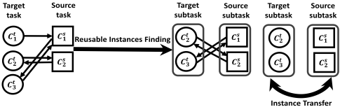
1) Reusable instances finding: this step is to find reusable instances in the source tasks for each target task. Generally if the tasks are related, there must exist some instances belonging to the same topic among these tasks. Therefore, for each target task, if we find the related clusters in its source tasks, the instances in the related clusters are considered reusable to the target task. To find the related clusters, we compute the distance of any two clusters between the target and source tasks through a commonly used symmetric and bounded distribution measure, i.e., the Jensen-Shannon divergence. Then based on the assumption that only the clusters closest to each other are possibly related, a pair of target and source subtasks which consist of the possibly related clusters are obtained, and instance knowledge is only transferred between the source and target subtasks. We give an illustration of the reusable instances finding process in Figure 1.
2) Subtask relatedness learning: this step is to further explore the relatedness of the constructed subtasks based on the first step. We use kernel mean matching to estimate the relatedness between them. Kernel mean matching is a method for estimating the mathematical expectation of a particular distribution by a weighted average of instances from another distribution. In other words, given a pair of target subtask and source subtask, kernel mean matching actively selects representative (positive weighted) instances from the source subtask to estimate the expectation of the target subtask distribution, which means that these selected representative instances in the source subtask are potentially relevant to the target subtask. Thus the relatedness of the source subtask to the target subtask can be estimated by the ratio of representative instances in the source subtask.
3) Clustering through instance transfer: this step is to cluster each target task by exploiting useful instance information from its source tasks. We construct a similarity matrix for each target task, with the similarity between any two data points to be the normalized weighted number of shared nearest neighbors from the target task itself and its source tasks. For each data point in the target task, if it is in the target subtask, its nearest neighbors are computed in both the target task itself and the corresponding source subtask; otherwise, its nearest neighbors are computed only in the target task itself. Then we adopt the Normalized Cut spectral clustering [Shi and Malik, 2000] to cluster each target task according to the learned similarity matrix. Through such a similarity construction, not only the useful instance information from all the tasks is used, but the independence of the clustering for each task is also ensured.
3.3 Reusable Instances Finding
For each target task Xt , we are going to find the related clusters from each source task Xs , and only the instances in the related clusters of the source task Xs are considered reusable to the target task Xt . We compute the distance of any two clusters between the target task Xt and source task Xs through Jensen-Shannon divergence [Lin, 1991].
where PCt i and PCs j are the probability distributions of cluster i in the target task Xt and cluster j in the source task Xs respectively, D(P♣♣Q) denotes the Kullback-Leibler divergence [Kullback and Leibler, 1951] between two probability distributions P and Q. For continuous probability distributions P and Q with the variable x in a domain D, the Kullback-Leibler divergence is defined as
where f(x) and g(x) are the probability density functions of the probability distributions P and Q. D(P♣♣Q) can also be expressed as
which is the expectation of the logarithmic difference between the distributions P and Q. Given a sample set B from distribution P, according to the law of large numbers and Eq.(3) [Jiang et al., 2013], D(P ♣♣Q) can be estimated by
We estimate the probability density functions fCt i (x) and fCs j (x) of the probability distributions PCt i and PCs j by kernel density estimation [Silverman, 1986]. In kernel density estimation, kernels are used to estimate the probability density function of a random variable. We use the most common Gaussian kernel in this paper, then we get the probability density function fCt i (x) in Eq.(5).
where x = (x▷D1↪ x▷D2↪ ▷ ▷ ▷ ↪ x▷Dd)T is a d-dimensional sample, the bandwidth hj which determines the amount of smoothing is set as hj = 1▷06 ⇥ δ♣C t i ♣- 15 according to the Silverman's rule of thumb [Silverman, 1986], δ is the standard deviation of the samples of C t i .
After computing the distance of any two clusters between each pair of target task Xt and source task Xs through Jensen-Shannon divergence in Eq.(1), we construct each pair of target subtask Z t and source subtask Z s by only retaining the clusters closest to each other.
3.4 Subtask Relatedness Learning
We exploit kernel mean matching [Huang et al., 2006] to learn the relatedness between each pair of target subtask Z t and source subtask Z s . To estimate the mathematical expectation of the distribution of the target subtask Z t by a weighted average of instances from its source subtask Z s , we have
where β 2 R˜ns is a reweighting factor for the source subtask Z s . zs i and zt j are the data points in the source subtask Z s and the target subtask Z t respectively, ˜ns and ˜nt are the numbers of data points in the source subtask Z s and the target subtask Z t respectively. Eq.(6) can be rewritten as
where Ks(i↪ j) = ⌦φ(zs i )↪ φ(zs j )↵ is the element in the matrix
tor st. Eq.(7) is a quadratic program which can be solved by the off-the-shelf quadratic programming solver in MATLAB. However, when the number of the processed data is large, it is computationally expensive. Fortunately, Eq.(7) can be solved efficiently by the Frank-Wolfe algorithm [Wen et al., 2015].
After β is calculated, we estimate the relatedness R(t) s of the source subtask Z s to the target subtask Z t by the ratio of positive weighted instances in the source subtask Z s by Eq.(8). Note that the relatedness metric in Eq.(8) is asymmetric, i.e., R(t) s 6= R(s) t .
3.5 Clustering through Instance Transfer
For each target task Xt , we construct a similarity matrix W t with the similarity between any two data points xti and xtj to be the normalized weighted number of shared nearest neighbors. The reusable instances are transferred to take part in the calculation of the nearest neighbors. Then we perform the Normalized Cut spectral clustering on each target task Xt according to the similarity matrix W t . To construct W t , for each data point xti in the target task Xt , we compute its nearest neighbors as follows. For each source task Xs :
1) If xti is in the target subtask Z t , its nearest neighbors consist of two parts: the nearest neighbors in the target task Xt itself, and the nearest neighbors in the source subtask Z s . To compute the nearest neighbors N (t) t (xti ) in the target task Xt itself, we choose the distance measurement that adapts to the data set to compute k(t) t nearest neighbors from Xt (e.g., for document data sets, we could choose cosine similarity, while for music analysis, we could choose the ItakuraSaito divergence), where k(t) t is a parameter to determine the number of nearest neighbors in Xt . To compute the nearest neighbors N (t) s (xti ) in the source subtask Z s , we map the data points in the target subtask Z t and the source subtask Z s to a same feature space, i.e., the Reproducing Kernel Hilbert Space H. Then we use the kernel trick (Gaussian kernel similarity) to compute k(t) s nearest neighbors fromZ s , where k(t) s is a parameter to determine the number of nearest neighbors in Z s . 2) If xti is not in the target subtask Z t , its nearest neighbors are computed only in the target task Xt itself. We choose the distance measurement that adapts to the data set to compute the nearest neighbors set N (t) t (xti ) which contains k(t) t nearest neighbors from Xt . And we set N (t) s (xti ) = ; since there are no related instances in the source task Xs .
Similar to the Shared Nearest Neighbor similarity, the similarity between xti and xtj is calculated by
Algorithm 1 SAMTC
- 1: Input: T tasks ¶Xt ♦Tt=1 , clustering numbers of all tasks ¶ht♦Tt=1 , the number of nearest neighbors k(t) s (s↪ t = 1↪ 2↪ ▷ ▷ ▷ ↪ T). Initialize the partitions of each task Xt : Ct = ¶Ct1 ↪ Ct2 ↪ ▷ ▷ ▷ ↪ Ctht ♦ by the Normalized Cut spectral clustering method with the Shared Nearest Neighbor similarity.
2: Output: Partitions ¶C(t) ♦Tt=1 . 3: for t = 1 to T do 4: for s = 1 to T do 5: if s 6= t then 6: Reusable Instances Finding: 7: Compute the distance between any two clusters Ct i and Cs j by Eq.(1). 8: Construct the target subtask Zt and the source subtask Zs with the instances in the clusters closest to each other. 9: Subtask Relatedness Learning: 10: Compute the relatedness R(t) s of the source subtask Zs to the target subtask Zt by Eq.(8). 11: Clustering through Instance Transfer: 12: Compute N (t) s (xti ) by Gaussian kernel similarity if xti 2 Zt , where N (t) s (xti ) is the set of k(t) s nearest neighbors in Zs for xti . 13: end if 14: end for 15: end for 16: Clustering through Instance Transfer: 17: for t = 1 to T do 18: Compute N (t) t (xti ) which contains k(t) t nearest neighbors inXt for xti . 19: Construct a similarity matrixW t by Eq.(9). 20: Apply the Normalized Cut spectral clusteringmethod to get the partitionC(t) . 21: end forif xti 2 N (t) t (xtj ) and xtj 2 N (t) t (xti ), otherwise we set W t (xti ↪ xtj ) = 0. In Eq.(9), R(t) s is computed by Eq.(8) when t 6= s, otherwise we set R(t) t = 1. share(t) s (xti ↪ xtj ) = N (t) s (xti ) T N (t) s (xtj ) is the set of shared nearest neighbors in the task Xs between xti and xtj if xti 2 N (t) t (xtj ) and xtj 2 N (t) t (xti ), otherwise share(t) s (xti ↪ xtj ) = ;. union(t) s (xti ↪ xtj ) = N (t) s (xti ) S N (t) s (xtj ) is the set of combined nearest neighbors in the task Xs between xti and xtj if xti 2 N (t) t (xtj ) and xtj 2 N (t) t (xti ), otherwise union(t) s (xti ↪ xtj ) = ;. The denominator in Eq.(9) is to normalize the weighted number of shared nearest neighbors. Since for each pair of data points xti and xtj , if either of them is not in the target subtask Z t , the numerator in Eq.(9) which represents the weighted number of shared nearest neighbors between them will be much smaller than that between the data points which are both in the target subtask Z t .
In summary, the overall process of the proposed SAMTC algorithm is listed in Algorithm 1. Denote d as the feature number, n as the sample number, the overall time complexity of SAMTC is O(n3 +n2d), which is comparable to the existing multi-task clustering methods. Moreover, the large-scale spectral clustering methods such as [Chen and Cai, 2011] can be applied to SAMTC to deal with large-scale data.
4 Experiments
4.1 Baselines and EvaluationMetrics
We compare the SAMTC method with typical single-task clustering methods k-means and Normalized Cut spectral clustering with Shared Nearest Neighbor similarity (NcutSNN) [Shi and Malik, 2000], which is a single-task version of SAMTC. We also compare SAMTC with the multi-task clustering methods which work for completely related tasks: the shared subspace learning multi-task clustering (LSSMTC) method [Gu and Zhou, 2009] and the convex discriminative multi-task feature clustering (MTFC) method [Zhang, 2015]. More importantly, we compare SAMTC with the multi-task clustering methods which work for partially related tasks: the smart multi-task clustering (S-MBC and S-MKC) methods [Zhang and Zhang, 2013], and the convex discriminative multi-task relationship clustering (MTRC) method [Zhang, 2015]. In addition, we evaluate SAMTC without using the Reusable Instances Finding term (SAMTC-nr) and the Subtask Relatedness Learning term (SAMTC-ns) respectively.
| Data set | Task id | Categories(#Sample) | #Feature | |||
|---|---|---|---|---|---|---|
| WebKB-c | Task 1 Task 2 Task 3 Task 4 | C1: Cornell.course(44) C1: Texas.course(38) C1: Washington.course(77) C1: Wisconsin.course(85) | C2: Cornell.faculty(34) C2: Texas.faculty(46) C2: Washington.faculty(31) C2: Wisconsin.faculty(42) | C3: Cornell.project(20) C3: Texas.project(20) C3: Washington.project(21) C3: Wisconsin.project(25) | C4: Cornell.student(127) C4: Texas.student(146) C4: Washington.student(126) C4: Wisconsin.student(154) | 2500 2500 2500 2500 |
| WebKB-p1 | Task 1 Task 2 Task 3 Task 4 | C1: Cornell.faculty(34) C1: Texas.course(38) C1: Washington.course(77) C1: Wisconsin.course(85) | C2: Cornell.project(20) C2: Texas.project(20) C2: Washington.faculty(31) C2: Wisconsin.faculty(42) | C3: Cornell.student(127) C3: Texas.student(146) C3: Washington.student(126) C3: Wisconsin.project(25) | 2500 2500 2500 2500 | |
| WebKB-p2 | Task 1 Task 2 Task 3 | C1: Cornell.faculty(34) C1: Texas.course(38) C1: Washington.course(77) C1: Wisconsin.course(85) | C2: Cornell.project(20) C2: Texas.project(20) C2: Washington.student(126) C2: Wisconsin.faculty(42) | C3: Texas.student(146) | 2500 2500 2500 2500 | |
| NG-p1 | Task 4 Task 1 Task 2 | C1: Comp.sys.ibm.pc.hw(392) C1: Rec.sport.hockey(399) | C2: Rec.sport.baseball(396) C2: Sci.space(392) | C3: Wisconsin.project(25) C3: Sci.med(392) C3: Talk.religion.misc(250) | 3000 3000 | |
| NG-p2 | Task 1 Task 2 | C1: Comp.graphics(387) C1: Comp.os.ms-win.misc(391) | C2: Rec.auto(395) C2: Rec.motocycle(397) | C3: Sci.crypt(395) C3: Sci.electronics(393) | C4: Talk.politic.mideast(376) | 3000 3000 |
| Reuters-p1 | Task 1 Task 2 Task 3 | C1: Economic index.gnp(63) C1: Economic index.cpi(60) C1: Economic index.ipi(36) | C2: Energy.crude(321) C2: Energy.nat gas(33) C2: Metal.copper(44) | C3: Food.cocoa(53) C3: Metal.iron steel(37) C3: Food.sugar(114) | 8121 8121 8121 | |
We adopt two performance measures in [Xu et al., 2003]: clustering accuracy (Acc) and normalized mutual information (NMI) to evaluate the clustering results.
4.2 Data Sets
We use data sets WebKB4, 20NewsGroups and Reuters 1 to construct the multi-task data sets in three typical cases (Table 1). The first case is that the tasks are completely related. We construct WebKB-c to represent this case. The second case is that the tasks are partially related and the cluster numbers in all the tasks are the same. We construct WebKB-p1, NGp1 and Reuters-p1 to represent this case. The third case is that the tasks are partially related and the cluster numbers in all the tasks are not the same. We construct WebKB-p2 and NG-p2 to represent this case.
4.3 Parameter Setting
For the parameters, we apply grid searching [Gu and Zhou, 2009] to identify the optimal values. For SAMTC, the number of nearest neighbors k(t) s (s 6= t) is set by searching the grid ¶ceil( ˜ns 2⇥˜hs )↪ ceil( ˜ns ˜hs )↪ min(ceil( 2⇥˜ns ˜hs )↪ ˜ns )♦, where ˜ns and ˜hs are the numbers of data points and clusters in the source subtask Z s respectively; the distance measurement during computing the nearest neighbors N (t) t (xti )
1 http://www.cad.zju.edu.cn/home/dengcai/Data/TextData.html
is cosine similarity. For SAMTC and Ncut-SNN, the number of nearest neighbors k(t) t is set by searching the grid ¶ceil( nt 2⇥ht )↪ ceil( nt ht )↪ min(ceil( 2⇥nt ht )↪ nt - 1)♦. For SMKC and SAMTC, the Gaussian kernel bandwidth is the median Euclidean distance between the data points. For S-MBC, the Bregman divergence we choose is Euclidean distance. For LSSMTC, the parameter λ is searched from ¶0▷1↪ 0▷2↪ ▷ ▷ ▷ ↪ 0▷9♦, the dimensionality of the shared subspace is searched from ¶2↪ 4↪ 6↪ 8↪ 10♦. For MTFC and MTRC, λ1 and λ2 are both searched from ¶2-10 ↪ 2-8 ↪ ▷ ▷ ▷ ↪ 2-2 ♦. For SMBC and S-MKC, λ is searched from ¶0▷1↪ 0▷2↪ ▷ ▷ ▷ ↪ 1♦.
Since MTFC and MTRC are convex optimization methods, we perform them once under each parameter setting, and show the clustering results under the best parameter setting. For the other methods, we repeat each method 10 times under each parameter setting, and show the mean clustering results and the standard deviations under the best parameter setting. As LSSMTC, MTFC and MTRC can only apply to the case that the cluster numbers of all the tasks are the same, we perform them on WebKB-c, WebKB-p1, NG-p1 and Reuters-p1.
4.4 Clustering Results
From the clustering results shown in Table 2 and Table 3, the following observations could be made.
1. SAMTC performs better than the single-task clustering methods such as k-means and Ncut-SNN, since SAMTC exploits the information across the related subtasks, whereas the single-task clustering methods only utilize the information within each task.
2. LSSMTC and MTFC always perform better than the single-task clustering methods on WebKB-c, whereas they may perform worse than the single-task clustering methods on the other data sets. This is because that LSSMTC and MTFC work for completely related tasks such as WebKB-c. For the other data sets in which the tasks are partially related, they may suffer from negative transfer.
3. S-MBC and S-MKC generally perform worse than the other multi-task clustering methods, because they require the distributions of the tasks to be the same or similar (and the more similar, the better), but the task distributions in the tested data sets do not show very high similarity.
| Data set | Task.Eval. | k-means | Ncut-SNN | LSSMTC | MTFC | MTRC | S-MBC | S-MKC | SAMTC-nr | SAMTC-ns | SAMTC |
|---|---|---|---|---|---|---|---|---|---|---|---|
| WebKB-c | T1.Acc(%) | 61.4◦ 2.6 | 59.5◦ 7.3 | 63.1◦ 6.2 | 75.1 | 40.9 | 57.9◦ 8.4 | 47.0◦ 2.2 | 66.7◦ 3.8 | 69.6◦ 5.0 | 71.5◦ 6.4 |
| T1.NMI(%) | 16.2◦ 3.4 | 27.7◦ 5.9 | 27.9◦ 3.9 | 38.3 | 13.6 | 25.0◦ 2.8 | 19.8◦ 4.1 | 36.6◦ 2.8 | 36.0◦ 4.6 | 39.4◦ 3.1 | |
| T2.Acc(%) | 48.7◦ 7.5 | 56.6◦ 7.5 | 63.0◦ 4.2 | 68.8 | 45.6 | 63.8◦ 7.4 | 45.1◦ 4.5 | 68.8◦ 4.0 | 69.2◦ 6.3 | 70.3◦ 4.8 | |
| T2.NMI(%) | 13.1◦ 4.4 | 25.2◦ 7.2 | 27.6◦ 2.2 | 36.8 | 17.0 | 27.0◦ 2.2 | 22.8◦ 4.3 | 38.6◦ 4.7 | 39.4◦ 6.6 | 40.0◦ 8.8 | |
| T3.Acc(%) | 53.9◦ 3.2 | 52.5◦ 5.1 | 57.5◦ 5.5 | 62.4 | 60.0 | 57.8◦ 5.4 | 49.3◦ 5.9 | 58.3◦ 2.7 | 60.1◦ 6.8 | 66.3◦ 6.1 | |
| T3.NMI(%) | 11.8◦ 3.4 | 26.1◦ 7.9 | 27.2◦ 4.5 | 30.0 | 46.6 | 26.7◦ 3.4 | 23.7◦ 7.2 | 30.3◦ 2.5 | 31.7◦ 6.4 | 35.3◦ 2.8 | |
| T4.Acc(%) | 60.5◦ 6.0 | 65.7◦ 6.5 | 68.9◦ 8.0 | 71.2 | 55.9 | 70.8◦ 6.6 | 52.9◦ 3.7 | 71.9◦ 3.9 | 73.1◦ 4.4 | 76.1◦ 5.5 | |
| T4.NMI(%) | 21.2◦ 10.6 | 35.1◦ 5.8 | 36.5◦ 4.1 | 49.4 | 36.9 | 39.4◦ 5.5 | 31.4◦ 3.1 | 47.9◦ 5.3 | 48.1◦ 3.7 | 49.4◦ 4.8 | |
| WebKB-p1 | T1.Acc(%) | 62.2◦6.9 | 60.4◦ 3.9 | 65.3◦ 4.2 | 65.2 | 48.6 | 67.2◦ 1.8 | 46.2◦ 2.8 | 67.6◦ 4.4 | 68.8◦ 4.0 | 74.5◦ 5.1 |
| T1.NMI(%) | 12.9◦ 5.7 | 13.2◦ 2.7 | 8.2◦ 4.0 | 21.6 | 19.3 | 10.0◦ 4.9 | 11.2◦ 2.1 | 19.0◦ 3.2 | 18.0◦ 4.1 | 22.5◦ 5.1 | |
| T2.Acc(%) | 69.5◦ 9.3 | 69.7◦ 3.1 | 70.2◦ 1.3 | 57.4 | 54.9 | 75.8◦ 1.6 | 50.8◦ 5.7 | 78.5◦ 4.9 | 75.9◦ 3.1 | 80.7◦ 7.5 | |
| T2.NMI(%) | 15.6◦ 4.4 | 42.0◦ 4.1 | 29.0◦ 3.4 | 36.3 | 14.2 | 34.7◦ 6.2 | 19.5◦ 8.6 | 47.8◦ 5.5 | 46.4◦ 4.1 | 53.6◦ 7.4 | |
| T3.Acc(%) | 57.3◦ 4.7 | 71.1◦ 2.4 | 65.6◦ 4.0 | 59.0 | 76.9 | 64.7◦ 6.3 | 59.5◦ 1.9 | 74.3◦ 0.8 | 76.1◦ 0.0 | 79.1◦ 0.0 | |
| T3.NMI(%) | 11.7◦ 7.6 | 36.2◦ 2.8 | 30.6◦ 3.2 | 33.4 | 53.5 | 29.7◦ 4.1 | 32.2◦ 2.9 | 39.0◦ 2.1 | 42.0◦ 0.0 | 44.2◦ 0.0 | |
| T4.Acc(%) | 52.8◦ 6.4 | 76.8◦ 3.8 | 76.6◦ 2.1 | 78.3 | 58.6 | 74.5◦ 4.6 | 65.1◦ 5.1 | 81.4◦ 1.6 | 83.6◦ 1.8 | 84.3◦ 1.0 | |
| T4.NMI(%) | 10.8◦ 2.8 | 53.0◦ 3.6 | 52.4◦ 4.1 | 46.3 | 47.0 | 50.4◦ 6.6 | 37.8◦ 3.3 | 58.1◦ 1.3 | 63.5◦ 3.6 | 64.5◦ 3.1 | |
| NG-p1 | T1.Acc(%) | 35.6◦ 0.5 | 72.7◦ 2.5 | 42.8◦ 2.2 | 85.2 | 92.7 | 44.9◦ 3.3 | 63.6◦ 2.9 | 83.7◦ 5.9 | 82.3◦ 5.4 | 86.6◦ 0.3 |
| T1.NMI(%) | 6.2◦ 1.6 | 47.8◦ 5.9 | 13.5◦ 1.4 | 55.0 | 72.4 | 19.0◦ 2.0 | 31.2◦ 2.9 | 57.7◦ 4.3 | 55.7◦ 3.6 | 60.3◦ 1.0 | |
| T2.Acc(%) | 33.8◦ 2.0 | 75.6◦ 4.1 | 53.8◦ 12.5 | 68.1 | 79.3 | 76.6◦ 10.1 | 62.2◦ 7.9 | 79.6◦ 4.8 | 80.3◦ 3.7 | 83.9◦ 1.4 | |
| T2.NMI(%) | 16.7◦ 2.3 | 50.1◦ 6.1 | 16.4◦ 13.3 | 35.1 | 43.1 | 41.8◦ 10.2 | 34.2◦ 6.5 | 54.0◦ 5.4 | 54.4◦ 4.6 | 57.3◦ 3.8 | |
| Reuters-p1 | T1.Acc(%) | 73.9◦ 8.7 | 80.0◦ 8.0 | 73.8◦ 11.3 | 81.2 | 60.0 | 80.0◦ 9.0 | 68.0◦ 2.9 | 83.6◦ 9.6 | 82.4◦ 7.0 | 86.8 ◦ 7.4 |
| T1.NMI(%) | 27.7◦ 17.8 | 58.8◦ 12.3 | 46.4◦ 2.7 | 16.1 | 34.6 | 56.6◦ 2.2 | 42.4◦ 1.4 | 62.8◦ 12.3 | 59.8◦ 10.5 | 63.1◦ 12.4 | |
| T2.Acc(%) | 61.8◦ 14.9 | 88.9◦ 10.0 | 87.9◦ 12.2 | 93.1 | 81.5 | 88.2◦ 12.2 | 91.3◦ 2.6 | 86.5◦ 1.0 | 81.5◦ 6.0 | 93.2◦ 1.2 | |
| T2.NMI(%) | 39.2◦ 25.4 | 72.7◦ 12.1 | 75.0◦ 13.9 | 75.8 | 64.1 | 74.5◦ 11.1 | 74.4◦ 6.4 | 62.0◦ 2.3 | 55.4◦ 0.9 | 77.3 ◦ 4.0 | |
| T3.Acc(%) | 65.0◦ 10.3 | 87.3◦ 10.6 | 77.1◦ 12.7 | 93.1 | 81.5 | 80.6◦ 10.6 | 69.2◦ 7.9 | 91.2◦ 5.3 | 90.9◦ 7.2 | 94.4◦ 3.5 | |
| T3.NMI(%) | 30.4◦ 18.6 | 67.5◦ 19.7 | 50.9◦ 15.1 | 75.8 | 64.1 | 56.7◦ 12.7 | 42.9◦ 8.6 | 74.4◦ 9.8 | 77.8◦ 5.7 | 82.0◦ 7.1 |
| Data set | Task.Eval. | k-means | Ncut-SNN | S-MBC | S-MKC | SAMTC-nr | SAMTC-ns | SAMTC |
|---|---|---|---|---|---|---|---|---|
| WebKB-p2 | T1.Acc(%) | 61.5◦ 4.5 | 71.5◦ 5.9 | 64.6◦ 0.6 | 64.3◦ 2.3 | 73.5◦ 4.3 | 72.8◦ 4.1 | 75.6◦ 0.8 |
| T1.NMI(%) | 5.8◦ 4.9 | 13.6◦ 8.1 | 6.9◦ 2.3 | 7.2◦ 2.8 | 15.8◦ 6.9 | 14.0◦ 5.2 | 20.2◦ 1.6 | |
| T2.Acc(%) | 69.5◦ 8.8 | 76.3◦ 3.9 | 80.0◦ 1.9 | 52.9◦ 3.2 | 77.2◦ 6.4 | 75.7◦ 7.1 | 80.6◦ 6.5 | |
| T2.NMI(%) | 14.7◦ 2.9 | 46.2◦ 5.4 | 34.6◦ 5.0 | 20.7◦ 6.0 | 49.7◦ 8.9 | 48.1◦ 6.5 | 50.9◦ 8.3 | |
| T3.Acc(%) | 63.6◦ 2.8 | 90.7◦ 0.7 | 88.4◦ 2.1 | 84.1◦ 1.4 | 92.0◦ 0.6 | 93.6◦ 1.2 | 93.9◦ 0.5 | |
| T3.NMI(%) | 5.1◦ 4.2 | 62.2◦ 2.3 | 49.5◦ 6.0 | 35.5◦ 2.7 | 59.9◦ 2.6 | 65.2◦ 4.4 | 66.5◦ 1.8 | |
| T4.Acc(%) | 53.6◦ 8.3 | 78.4◦ 1.9 | 76.6◦ 3.0 | 62.8◦ 6.8 | 80.9◦ 2.4 | 79.1◦ 9.5 | 85.5◦ 0.0 | |
| T4.NMI(%) | 11.9◦ 11.0 | 59.8◦ 3.8 | 55.4◦ 5.7 | 37.9◦ 5.9 | 55.6◦ 4.6 | 60.0◦ 8.2 | 68.1◦ 0.0 | |
| NG-p2 | T1.Acc(%) | 36.4◦ 3.2 | 66.3◦ 4.2 | 45.6◦ 4.2 | 73.9◦ 1.2 | 68.7◦ 5.9 | 71.6◦ 6.2 | 78.3◦ 5.5 |
| T1.NMI(%) | 6.8◦ 3.5 | 36.9◦ 5.6 | 18.2◦ 10.9 | 37.5◦ 2.0 | 37.2◦ 5.5 | 41.2◦ 5.1 | 46.7◦ 4.8 | |
| T2.Acc(%) | 40.1◦ 2.2 | 65.3◦ 6.7 | 46.1◦ 4.1 | 66.6◦ 1.6 | 67.8◦ 3.5 | 66.0◦ 6.1 | 70.7◦3.9 | |
| T2.NMI(%) | 4.9◦ 4.1 | 36.9◦ 8.6 | 21.0◦ 5.4 | 40.0◦ 2.5 | 45.6◦ 3.2 | 44.4◦ 3.0 | 47.8◦ 4.5 |
4. The performance of MTRC is not so good as we expected and is quite unstable. It performs the best on the task 1 of NG-p1, but performs not so well on the task 2 of NGp1 and the other data sets. This is because that MTRC assumes that the label marginal distribution in each task distributes evenly, and only the task 1 of NG-p1 in the tested data sets satisfies such assumption. Moreover MTRC requires the cluster numbers of all the tasks to be same, which limits its applicability.
5. SAMTC-nr and SAMTC-ns perform better than NcutSNN in most cases, which illustrates that the Reusable Instances Finding term and the Subtask Relatedness Learning term are very essential to measure the relatedness among the tasks. But from the comparison of SAMTC with SAMTCnr and SAMTC-ns, it can be seen that using the two terms together can achieve better clustering performance than only using one term. SAMTC-nr and SAMTC-ns sometimes perform worse than Ncut-SNN, because only using one term cannot fully explore the relatedness among the tasks.
6. SAMTC generally performs much better than the compared multi-task clustering methods (except for the task 1 of NG-p1 on which it performs the second best, whereas MTRC performs the best), since SAMTC does not have the aforementioned limitations in the compared multi-task clustering methods, it tackles the partially related tasks by making the most of the reusable instance information while disregarding the uncorrelated instances, i.e., it can exploit the positive relatedness among the tasks and avoid negative transfer.
5 Conclusion
In this paper, we have proposed a general self-adapted multitask clustering (SAMTC) algorithm, which can exploit the positive relatedness among the tasks and avoid negative transfer by identifying the reusable instances between each pair of tasks. SAMTC first finds the reusable instances between each pair of tasks and obtains a pair of subtasks, then it further explores the relatedness between each pair of subtasks, finally it constructs the similarity matrix for each task by exploiting useful instance information from the other tasks through instance transfer and performs spectral clustering on the constructed similarity matrix. Experimental results on several real data sets show the superiority of the proposed algorithm over traditional single-task clustering methods and existing multi-task clustering methods.
Acknowledgments
This work was supported by National Science Foundation of China (No. 61272374,61300190,61428202) and National High Technology Research and Development Program (863 Program) of China (No. 2015AA015403).
@inproceedings{ijcai2016p336,
  title     = {Self-Adapted Multi-Task Clustering},
  author    = {Zhang, Xianchao and Zhang, Xiaotong and Liu, Han},
  booktitle = {Proceedings of the Twenty-Fifth International Joint Conference on
               Artificial Intelligence, {IJCAI-16}},
  publisher = {AAAI Press / International Joint Conferences on Artificial Intelligence},
  editor    = {Subbarao Kambhampati},
  pages     = {2357--2362},
  year      = {2016},
  month     = {7},
  url       = {https://ijcai.org/proceedings/2016/336},
}
TY - CPAPER TI - Self-Adapted Multi-Task Clustering AU - Zhang, Xianchao AU - Zhang, Xiaotong AU - Liu, Han T2 - Proceedings of the Twenty-Fifth International Joint Conference on Artificial Intelligence, IJCAI-16 PB - AAAI Press / International Joint Conferences on Artificial Intelligence PY - 2016 SP - 2357 EP - 2362 UR - https://ijcai.org/proceedings/2016/336 ER -Copied
Machine-readable versions of this paper, for tools and AI agents:





