
Bayesian Dictionary Learning with Gaussian Processes and Sigmoid Belief Networks
Proceedings of the Twenty-Fifth International Joint Conference on Artificial Intelligence. Pages 2364-2369.
Abstract
In dictionary learning for analysis of images, spatial correlation from extracted patches can be leveraged to improve characterization power. We propose a Bayesian framework for dictionary learning, with spatial location dependencies captured by imposing a multiplicative Gaussian process (GP) priors on the latent units representing binary activations. Data augmentation and Kronecker methods allow for efficient Markov chain Monte Carlo sampling. We further extend the model with Sigmoid Belief Networks (SBNs), linking the GPs to the top-layer latent binary units of the SBN, capturing inter-dictionary dependencies while also yielding computational savings. Applications to image denoising, inpainting and depth-information restoration demonstrate that the proposed model outperforms other leading Bayesian dictionary learning approaches.
- M. Aharon, M. Elad, and A. Bruckstein. K-SVD: An algo- rithm for designing overcomplete dictionaries for sparse representation. IEEE Transactions on Signal Processing, 54(11):4311-4322, 2006.
- H. M. Choi, J. P. Hobert, et al. The Polya-gamma Gibbs sam- pler for Bayesian logistic regression is uniformly ergodic. Electronic Journal of Statistics, 7:2054-2064, 2013.
- A. C. Damianou and N. D. Lawrence. Deep Gaussian pro- cesses. In AISTATS, 2013.
- S. Flaxman, A. G. Wilson, D. Neill, H. Nickisch, and A. J. Smola. Fast Kronecker inference in Gaussian processes with non-Gaussian likelihoods. In ICML, 2015.
- Z. Gan, C. Chen, R. Henao, D. Carlson, and L. Carin. Scal- able deep poisson factor analysis for topic modeling. In ICML, 2015a.
- Z. Gan, R. Henao, D. Carlson, and L. Carin. Learning deep sigmoid belief networks with data augmentation. In AIS- TATS, 2015b.
- P. Garrigues and B. A. Olshausen. Learning horizontal con- nections in a sparse coding model of natural images. In NIPS, 2007.
- Z. Ghahramani and T. L. Griffiths. Infinite latent feature mod- els and the Indian buffet process. In NIPS, pages 475-482, 2005.
- E. Gilboa, Y. Saatci, and J. P. Cunningham. Scaling multi- dimensional inference for structured Gaussian processes. IEEE Transactions on Pattern Analysis and Machine Intel- ligence, 37(2):424-436, 2015.
- H. He and W.-C. Siu. Single image super-resolution using Gaussian process regression. In CVPR. IEEE, 2011.
- J. Hensman, N. Fusi, and N. D. Lawrence. Gaussian pro- cesses for big data. In UAI, 2013.
- P. J. Liu. Using Gaussian process regression to denoise im- ages and remove artefacts from microarray data. PhD the- sis, University of Toronto, 2007.
- S. Lu, X. Ren, and F. Liu. Depth enhancement via low-rank matrix completion. In CVPR, 2014.
- J. Mairal, F. Bach, J. Ponce, and G. Sapiro. Online dictionary learning for sparse coding. In ICML, 2009.
- R. M. Neal. Bayesian Learning for Neural Networks. Springer, 1996.
- R. M. Neal. Monte carlo implementation of Gaussian process models for Bayesian regression and classification. Arxiv, 1997.
- K. B. Petersen and M. S. Pedersen. The matrix cookbook. Technical report, Technical University of Denmark, 2012.
- G. Polatkan, M. Zhou, L. Carin, D. Blei, and I. Daubechies. A Bayesian nonparametric approach to image super- resolution. IEEE Transactions on Pattern Analysis and Machine Intelligence, 37(2):346-358, 2015.
- N. G. Polson, J. G. Scott, and J. Windle. Bayesian infer- ence for logistic models using Pólya-gamma latent vari- ables. JASA, 108(504):1339-1349, 2013.
- C. E. Rasmussen and C. K. I. Williams. Gaussian Processes for Machine Learning. MIT Press, 2006.
- D. Scharstein and R. Szeliski. A taxonomy and evaluation of dense two-frame stereo correspondence algorithms. Inter- national Journal of Computer Vision, 2002.
- J. R. Shewchuk. An introduction to the conjugate gradient method without the agonizing pain. Technical report, Uni- versity of California at Berkeley, 1994.
- M. K. Titsias. Variational learning of inducing variables in sparse Gaussian processes. In AISTATS, 2009.
- C. Wachinger, P. Golland, M. Reuter, and W. Wells. Gaussian process interpolation for uncertainty estimation in image registration. In MICCAI. Springer, 2014.
- S. Wang, L. Zhang, and R. Urtasun. Transductive Gaussian processes for image denoising. In ICCP, 2014.
- Z. Xing, M. Zhou, A. Castrodad, G. Sapiro, and L. Carin. Dictionary learning for noisy and incomplete hyperspectral images. SIAM J. Imaging Sciences, 5(1):33-56, 2012.
- J. Yang, Z. Wang, Z. Lin, S. Cohen, and T. Huang. Coupled dictionary training for image super-resolution. IEEE Transactions on Image Processing, 21(8):3467- 3478, 2012.
- Z. Zhang. Microsoft kinect sensor and its effect. IEEE Mul- timedia, 19(2):4-10, 2012.
- M. Zhou, H. Chen, J. W. Paisley, L. Ren, L. Li, Z. Xing, D. B. Dunson, G. Sapiro, and L. Carin. Nonparametric Bayesian dictionary learning for analysis of noisy and incomplete images. IEEE Transactions on Image Processing, 21(1): 130-144, 2012.
- M. Zhou, H. Chen, L. Ren, G. Sapiro, L. Carin, and J. W. Paisley. Non-parametric Bayesian dictionary learning for sparse image representations. In NIPS, 2009.
- M. Zhou, H. Yang, and G. Sapiro. Dependent hierarchical beta process for image interpolation and denoising. In AIS- TATS, 2011.
References were extracted automatically from the PDF and may contain errors.
Full text extracted automatically from the PDF; figures, tables and equations may differ. The PDF is the version of record.
1 Introduction
Learning overcomplete sparse latent representations for signal restoration and characterization has recently led to stateof-the-art results in tasks such as image denoising, inpainting, super-resolution and compressive sensing (Zhou et al., 2009; Yang et al., 2012). Traditional approaches learn sparse codes from a fixed number of dictionary elements, while minimizing the reconstruction error subject to imposed sparsity regularization (Aharon et al., 2006; Mairal et al., 2009). Non-parametric Bayesian approaches have been introduced to tackle this challenge (Zhou et al., 2009, 2012; Polatkan et al., 2015) by employing methodologies like the Indian Buffet Process (IBP) (Ghahramani and Griffiths, 2005). Such Bayesian approaches provide a principled way to estimate uncertainty and typically yield excellent generalization ability.
Recent work has demonstrated that modeling images as a collection of sub-regions or patches is important, because leveraging local image structure is instrumental for representational quality (Mairal et al., 2009; Zhou et al., 2009). The key idea in this line of work is that similar patches are likely to share dictionary elements. Furthermore, dictionary learning can be greatly improved by imposing that patches close in space are likely to use the same or similar dictionary elements
(Zhou et al., 2011). Specifically, the dependent Hierarchical Beta Process (dHBP) (Zhou et al., 2011) utilizes a dependent IBP to capture spatial correlations, via a 2-D smoothing function based on patch locations. Although this approach leads to dramatic performance improvements, the smoothing function has to be specified parametrically, and the posterior of their Bayesian formulation is not locally conjugate, which makes inference challenging.
Gaussian Process (GP) priors (Rasmussen and Williams, 2006) are a natural choice for capturing spatial dependencies. Such priors provide a principled non-parametric way to estimate correlation as a function of relative spatial location. However, despite great flexibility, GPs are known to be computationally expensive; in fact, they become prohibitively expensive as the number of observations grows.
In this paper, we propose a framework for dictionary learning where patch-to-patch spatial dependencies are modeled via GP priors linked to binary dictionary element activations. Furthermore, we utilize deep Sigmoid Belief Networks (SBNs) to impose correlation structure across dictionary elements. We demonstrate that use of the SBN reduces the number of needed GP draws, thereby also manifesting significant computational acceleration.
The contributions from our framework are: (i) Gaussian process priors that capture spatial dependencies between patches in images; (ii) SBNs that capture dependencies between dictionary elements; (iii) efficient inference via Kronecker methods for GPs, and a fully local conjugate Bayesian formulation based on P´olya-gamma data-augmentation; (iv) computational savings by reducing the number of needed GPs, by linking them to the top layer of the SBN; (v) results on denoising, inpainting and depth restoration, that demonstrate the flexibility of our approach and highlight how learning dependency structure yields superior performance.
Related Work Several studies have employed GPs in tasks such as interpolation (Wachinger et al., 2014), superresolution (Wachinger et al., 2014; He and Siu, 2011) and denoising (Liu, 2007; Wang et al., 2014). These works are based on the insight that images composed of noisy or corrupted patches can be used to produce clean images as output, by leveraging statistical correlations between image patches. Similar patches are more likely to have same outputs. Our work is complementary to their work in that we use GPs for location dependencies, not patch similarities.
Other work has also explored GPs as priors for dictionary elements. Xing et al. (2012) characterized multi-channel hyper-spectral images, where each channel is associated with a distinct wavelength. Their assumption is that dictionary elements from different channels are smooth as a function of wavelength, whereas we assume that dictionary activation is a smooth function of location. Garrigues and Olshausen (2007) developed a method close to ours; they proposed a sparse coding model where spatial dependencies are imposed via pairwise coupling using an Ising model. However, their model requires a user-defined temperature parameter that uniquely controls the strength of coupling.
2 Background: Bayesian Dictionary Learning
Assume observed data X = ¶x1↪ ▷ ▷ ▷ ↪ xN♦ 2 J⇥N , where xi represents one of N patches extracted from a single image. In Bayesian dictionary learning, the goal is to learn dictionary elements, D = ¶d1↪ ▷ ▷ ▷ ↪ dM♦ 2 J⇥M from X. The i-th observations is represented as
where ⊙ denotes the Hadamard product, and IJ is the J ⇥ J identity matrix. Vectors wi = ¶wi1↪ ▷ ▷ ▷ ↪wiM♦ 2 M and zi = ¶zi1↪ ▷ ▷ ▷ ↪ ziM♦ 2 ¶0↪ 1♦M represent real weights and binary activations, respectively. Specifically, zi encodes which dictionary elements are used to represent xi, and "i is i.i.d. additive Gaussian noise (or model residual). Hyperpriors are placed on the variances of wi and "i, via inverseGamma distributions on σ2w and σ2 " , which enables us to share dispersion information across dictionary elements.
3 Dictionary Learning with Gaussian Processes
One possible approach to encourage sparsity in the binary activations, zi, is to use a Bernoulli-beta specification (Zhou et al., 2009), which assumes each zi is drawn i.i.d.. However, Zhou et al. (2011) demonstrated that it is reasonable to assume that patches located near each other are likely to be represented in terms of the same or similar dictionary elements, and thus binary activations of nearby patches are likely to be consistent with spatial dependencies. We incorporate such prior belief into (1) by means of a GP on a 2-D spatial field. Our approach differs from Zhou et al. (2011), in that GPs allow estimation of binary activation dependencies, by connecting the GP output to a logistic link function. We call our method Gaussian Process Factor Analysis (GP-FA). The construction for the m-th binary activation, zim becomes
where σ(·) denotes the sigmoid function, yim is the value of function fm(·) evaluated at the i-th patch, with the spatial coordinates of li = ¶l(1) i ↪ l(2) i ♦, where l(q) i denotes the coordinates of q-th dimension in 2D images. The function fm(·) is drawn from a GP with constant mean function, θm(·) = bm, and multiplicative covariance function, km(li↪ ·), defined as km(li↪ ·) = k(1) m (l(1) i ↪ ·) ⌦ k(2) m (l(2) i ↪ ·). For the mean, bm, we specify a Gaussian prior with mean and variance, λm and σ2 b :
To encourage sparsity in the activations, zim, we bias function instances, yim, towards negative values using a negativetruncated Gaussian distribution, denoted as N-, with variance σ2λ . Since this prior is shared by all factors, it encourages sparsity globally. Further, the hierarchy in (3) is convenient from a practical standpoint, because it yields local conjugacy.
For the covariance function, km(·↪ ·), we consider the widely used squared exponential (SE) function. Specifically, the covariance function for axis s = ¶1↪ 2♦, is defined as
where ⇥m = ¶(σ2 f )m↪ ✓m♦ is the set of parameters for the m-th dictionary element, (σ2 f )m is the signal variance and ✓m is the characteristic length scale (Rasmussen and Williams, 2006).
Note that in our covariance-function specification, we are assuming that the Gaussian process is isotropic in different spatial axes, s, provided that different dimensions share the same characteristic length scale, ✓m. This assumption may seem strong, but works well in practice (He and Siu, 2011). Since our covariance function is multiplicative and isotropic, the similarity between any two patches centered at li and li0 is based on the Euclidean distance between their centers.
P´olya-gamma augmentation Gaussian process priors linked to binary data as in (2) have been traditionally used for classification tasks. In such a scenario, the Laplace approximation or Expectation Propagation (EP) are typically employed to approximate the non-Gaussian posterior resulting from non-Gaussian likelihoods (Rasmussen and Williams, 2006). MCMC approaches have been proposed as well (Neal, 1997), but they are inefficient because the posterior distribution has to describe highly correlated variables. Here we employ Gibbs sampling, leveraging the P´olya-gamma (PG) data augmentation scheme of Polson et al. (2013). In contrast to probit-based augmentation, PG augmentation has been shown to be efficient with sophisticated posteriors (Gan et al., 2015b,a), while enjoying theoretical guarantees in terms of unbiased estimates of posterior expectations (Choi et al., 2013). Briefly, if the auxiliary variable γ is draw from P´olyagamma distribution, i.e., γ ⇠ PG(1↪ 0), the following identity holds for any
This identity enables one to write the joint distribution for zm = ¶z1m↪ ▷ ▷ ▷ ↪ zNm♦, ym = ¶y1m↪ ▷ ▷ ▷ ↪ yNm♦ and γm = ¶γ1m↪ ▷ ▷ ▷ ↪ γNm♦ as
which is convenient because it gives rise to closed-form conditional posteriors for zm, ym and γm.
Gibbs updates for each yim can be obtained by conditioning on the remaining y∩im , ym∩yim. In the following discussion, we use the notation K to denote the N ⇥ N Gram matrix of the Gaussian process obtained by evaluating km(li↪ ·) at ¶li♦Ni=1 , and we omit the dictionary index m for clarity. From (4) we obtain
where "-" denotes all conditioning parameters. Note that both K and y have been permuted to keep ki↪i on the lefttop corner of the matrix, for notational convenience. We adopt a patch-by-patch approach to sequentially sample all patches indexed by i. It is possible to sample sub-regions of adjacent patches simultaneously from a blocked multivariate Gaussian. However, sub-region size should be carefully selected or estimated from data. As an alternative to sampling, we could use fast variational methods for sparse GPs instead (Titsias, 2009; Hensman et al., 2013). We leave these possibilities as interesting future work.
The conditional posterior for binary activations, zim, is dependent on both dictionary factorization and Gaussian process prior, thus we can write
Kronecker method Unfortunately, the approach in (5) is costly, scaling as O(N 3 ) time and O(N 2 ) memory per patch, due to matrix inversion. As a result, it becomes prohibitive even when processing relatively small images, say where N = (256-8+1)2 , for a 256⇥256 image and patch size 8⇥8. Recently, efficient GP methods were proposed for both Gaussian (Gilboa et al., 2015) and non-Gaussian (Flaxman et al., 2015) likelihoods, by exploiting the Kronecker structure of multiplicative GPs. In this paper, we adopt the fast inference method of Gilboa et al. (2015), where the computational cost can be effectively reduced to O(N 3◁2 ) time and O(N) mem-
The approximation above allows us to perform a single inversion on the full Gram matrix, K, instead of K∩i↪∩i. This is desirable because K can be represented as K = K1 ⌦K2. Existing Kronecker methods can be applied via Preconditioned Conjugate Gradient (PCG) (Shewchuk, 1994), by solving the following linear system of equations
where P = Γ- 12 is the pre-conditioner matrix. The key idea behind (7) relies on the fast computation of Kroneckerproduct vector multiplication ↵ = (⌦Dd=1Ad)b (Gilboa et al., 2015). To further reduce computational cost, we ignore locations with negligible correlation w.r.t the current location, i.e., ⇢(i↪ i0 ) < 10-6 . This enables us to only consider a relatively small number of neighbor patches within radius R to the current location, as a consequence of the light tails of the SE covariance function. In practice, we found that the radius, R, is determined by the length scale of the GP, ✓, and is usually less than 20. Thanks to this approximation, the computation cost per patch is further reduced to O(R3 ) time.
Automatic relevance determination To estimate the parameters of the covariance functions, ¶⇥m♦Mm=1 , we use maximum a posterior (MAP) estimation for (σ2 f )m and ✓m, corresponding to dictionary element m. This is done by maximizing the conditional log-posterior function, Lm. Again, the Kronecker product trick can be employed for fast inference via Cholesky decompositions, denoted here as chol(·). The entire computation for one patch can be done in O(N 3◁2 ) time and O(N) memory. Omitting constant terms,
where v = ym¶(LT1 )-1 ⌦ (LT2 )-1 ♦ and L1 = chol(K(1) m ) and L2 = chol(K(2) m ). Note that parameters, ¶⇥m♦Mm=1 , are factor-wise independent, thus can be updated in parallel. p0 is the prior for (σ2 f )m and ✓m, specified as logN(0↪ 1) ⇥ logN(0↪ 1). Provided that we estimate individual characteristic length scales, ✓m for each factor, m, in a MAP context, our approach can be seen as an instance of automatic relevance determination (Neal, 1996).
Missing pixels In tasks such as inpainting, we are given images with missing pixels. As in Zhou et al. (2009), missing pixel values can be integrated out, thus inference can be performed w.r.t. observed pixels only. Further, we can impute missing values by treating them as latent variables to be estimated jointly with all the other parameters of the model, via closed-from conditional predictive distributions.
4 Leveraging the Sigmoid Belief Network
In (1), the GP is directly input to a sigmoid function, and therefore the number of GPs is equal to the number of dictionary elements. For large number of dictionary elements of typical interest, this may be computationally prohibitive. Additionally, each of the GPs are drawn independently, so in (1) there is no dependency imposed between the dictionary elements (it is likely that correlation in dictionary usage exists).
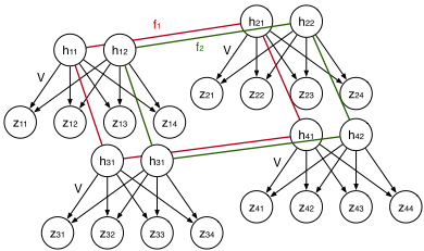
Both of these limitations are addressed by constituting a Sigmoid Belief Network (SBN), with the number of binary units at the bottom SBN layer equal to the number of dictionary elements (the bottom of the SBN replaces the sigmoid function in (1)). The SBN imposes correlation in dictionary usage. Further, the GPs are imposed at the top layer of the SBN, with one GP for each top-layer unit. Since the number of top-layer units is typically markedly smaller than that at the bottom SBN layer, this model significantly reduces the number of needed GPs. This model uses GPs to impose patch-dependent spatial correlation at the top of the SBN, and the multiple layers of the SBN impose correlation between dictionary-element usage (see Figure 1). We denote this model as GP-SBN-FA.
Building on recent SBN work (Gan et al., 2015b), we consider an SBN with L binary units at the top:
where a GP prior is placed on the spatial dependence of each component of yi = (yi1↪ ▷ ▷ ▷ ↪ yiL)T , and hi 2 ¶0↪ 1♦L is a vector of L binary units. The weight matrix, V 2 RM⇥L, contains L features encoding M dictionary elements correlations. We place a three-parameter beta normal prior on the weight matrix, V , which has demonstrated good mixing performance (Gan et al., 2015b). Further, we let b ⇠ N(0↪ IM), for simplicity. Closed-form conditional posteriors for ¶V ↪ b♦ via Gibbs sampling are available via P´olya-gamma data augmentation (Gan et al., 2015b). The conditional posterior for hi is very similar to that for zim in (6). In this work we only consider one-layer SBNs as in (8). However, adding layers to form deep architectures is straightforward, as previously described by Gan et al. (2015b).
It is likely that the number of SBN features, L, needed to describe correlations across dictionary elements is considerably smaller than the dictionary size, and therefore M < L. We have observed that L = M◁2 works well in practice.
Previous work has shown that one-layer SBNs with infinite number of hidden units can be explained as GPs (Neal, 1996). However, stacking GPs in multi-layer configurations such as that of Damianou and Lawrence (2013) can be prohibitive due to the high cost of GP inference. Our GP-SBN-FA can be seen as a way to combine the flexibility of GPs with the computational efficiency of SBNs, in a model where GPs are only used where they are most needed, in our case to capture spatial dependencies.
5 Experiments
We present experiments on two sets of images. The results on gray-scale images for denoising and inpainting tasks highlight how characterization of spatial structure improves results. Results on depth-information recovery demonstrates that our GP-based approach can improve the restoration of multi-channel images, by capturing channel dependencies.
5.1 2-DGrayscale Images
Denoising We analyzed 10 gray-scale images typically used to benchmark image denoising methods. We added isotropic i.i.d. Gaussian noise, N(0↪ σ), to each pixel with σ = 25 and 50 (the gray-scale pixel value range from 0 to 255). As input to our model, each image was partitioned into 8 ⇥ 8 patches with sliding distance of one pixel, i.e., the distance between centers of neighbor patches is one pixel. We ran 500 MCMC iterations with random initialization and kept the last 50 samples for image reconstruction (averaging over these collection samples). The hyper-parameters controlling Gaussian distribution variances, i.e., σb and σλ, were all set to 0▷1. As suggested in Zhou et al. (2009), the hyper-parameters for the inverse Gamma distributions (the priors for σw and σ") were set to ¶10-6 ↪ 10-6 ♦. Dictionary sizes in both GPFA and GP-SBN-FA are initially set to 128. In GP-SBN-FA, we use a one-layer SBN with the number of top-layer binary units L set to half the size of the dictionary M. For each MCMC iteration, computations were parallelized w.r.t. dictionary elements using a desktop GPU. We use Peak Signalto-Noise Ratio (PSNR) to measure the recovery performance of original images. Compared with BPFA (Zhou et al., 2009), as shown in Table 1, GP-SBN-FA yields the best results for most images under different noise regimes. The performance of dHBP (Zhou et al., 2011) is similar to BPFA but no better than GP-FA or GP-SBN-FA, thus not shown.
Inpainting We performed image inpainting on the same gray-scale images from the previous experiment, where a portion of pixels were set to missing (selected uniformly at random). The dictionary size M is set as either 256 or 512, to match image size. Other hyper-parameters are set as in the denoising task. We consider two observed pixel ratios, 20% and 50%. 500 MCMC iterations were used, and 50 samples were collected for reconstruction. In this task, we compared with dHBP and BPFA; results and experiment settings for dHBP were obtained from Zhou et al. (2011). The results on 50% observed data are shown in Table 2. GP-FA and GP-SBN-FA can generally yield better PSNR than dHBP when the proportion of observed data is relatively high, 50%. When this proportion drops to 20%, dHBP tends to outperform our approach. We hypothesize that lower observed proportions may lead to poor estimation of the GP posterior, where a predefined filtering function with domain knowledge such as that of dHBP may be favorable.
| σ = 25 | |||||
|---|---|---|---|---|---|
| Method | C.man | House | Pepper | Lena | Barbara |
| BPFA | 28.41 | 31.92 | 29.36 | 31.25 | 28.83 |
| GP-FA | 28.70 | 32.22 | 29.65 | 31.42 | 29.11 |
| GP-SBN-FA | 28.99 | 32.23 | 29.78 | 31.51 | 29.18 |
| Method | Boats | F.print | Man | Couple | Hill |
| BPFA | 29.25 | 27.44 | 29.06 | 28.89 | 29.29 |
| GP-FA | 29.49 | 27.55 | 29.27 | 29.04 | 29.49 |
| GP-SBN-FA | 29.56 | 27.54 | 29.23 | 29.15 | 29.52 |
| σ = 50 | |||||
| Method | C.man | House | Pepper | Lena | Barbara |
| BPFA | 24.31 | 27.62 | 25.41 | 27.59 | 25.14 |
| GP-FA | 24.66 | 28.12 | 25.71 | 27.80 | 25.44 |
| GP-SBN-FA | 24.66 | 28.15 | 25.67 | 27.83 | 25.39 |
| Method | Boats | F.print | Man | Couple | Hill |
| BPFA | 25.72 | 23.80 | 25.95 | 25.37 | 26.25 |
| GP-FA | 25.99 | 23.91 | 26.22 | 25.51 | 26.48 |
| GP-SBN-FA | 26.03 | 23.89 | 26.18 | 25.45 | 26.45 |
| Method | C.man | House | Pepper | Lena | Barbara |
|---|---|---|---|---|---|
| BPFA | 28.90 | 38.02 | 32.58 | 36.94 | 33.17 |
| dHBP | 29.89 | 38.83 | 32.90 | 37.14 | 36.03 |
| GP-FA | 29.03 | 38.53 | 32.84 | 37.18 | 33.18 |
| GP-SBN-FA | 28.98 | 38.89 | 33.04 | 37.01 | 33.33 |
| Method | Boats | F.print | Man | Couple | Hill |
| BPFA | 33.78 | 33.53 | 33.29 | 35.56 | 34.23 |
| dHBP | 33.92 | 32.70 | 33.72 | 33.54 | 34.14 |
| GP-FA | 34.16 | 34.08 | 33.83 | 34.63 | 34.46 |
| GP-SBN-FA | 33.98 | 33.89 | 33.54 | 33.60 | 34.31 |
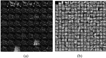
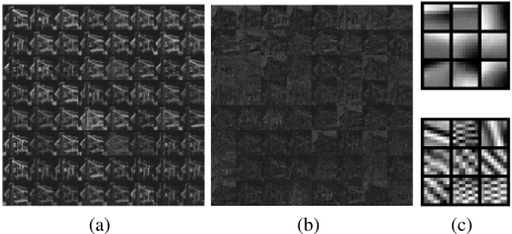
The learned dictionary elements and binary activations for dictionary elements, obtained from 50% observed data and GP-FA, are shown in Figure 2(a,b). The binary activation patterns of GP-SBN-FA for each dictionary, as seen in Figure 3(a), seem to be more similar with each other, compared to those from GP-FA, as in Figure 2(a). For GP-SBN-FA, the binary units of SBN, that capture co-occurrence of dictionary elements, are also shown in Figure 3(b). Both GP-FA and GP-SBN-FA effectively capture spatial dependencies by incorporating GP priors. One interesting observation is that the imposed SBN architecture encourages blocks of dictionary elements that share similar patterns to simultaneously turn on or turn off, as shown in Figure 3(c). Such an interdictionary dependency assumption is useful when the dictionary elements are heavily correlated.
All the experiments were conducted on a single machine with two 2▷7 GHz processors and 12 GB RAM. The computations of M GPs in GP-FA (or L GPs in GP-SBN-FA) were parallelized using a GPU, rendering the running time of GPFA and GP-SBN-FA comparable with dHBP. For a 256⇥256 image, one single iteration of GP-FA takes 96 seconds, while GP-SBN-FA takes 68 seconds (code written in Matlab and C++). When doubling the number of MCMC iterations, the average PSNR for our method increases by approximately 0▷15 dB for both GP-FA and GP-SBN-FA in the inpainting tasks, suggesting that taking more iterations may marginally improve results.
5.2 Depth Restoration
Modern depth cameras (Zhang, 2012) capture color and depth (RGB-D) information of a scene. However, depth maps captured by these devices are often noisy and miss pixel values, especially around object boundaries (Lu et al., 2014). Here we extend our Bayesian approach for the joint learning of multi-channel images applied to RGB-D image restoration.
We extend the covariates for patch i as li 2 ¶l(1) i ↪ l(2) i ↪ l(c) i ♦, where l(c) i = ¶R↪G↪B↪D♦ indicates the channel of patch i. Prior domain knowledge suggests that depth-to-RGB correlation is lower than correlation within RGB channels (Lu et al., 2014). To leverage such prior information, we use ✓dm to describe the relative depth-to-RGB dissimilarity. We also let ✓cm be the characteristic length scale of the third-dimension covariance function, kcm. The covariance function, represented in Gram matrix, is defined as Km = K(1) m ⌦K(2) m ⌦K(c) m . Specifically,
Conceptually, when determining whether a certain dictionary element is activated on a certain patch, the model seeks dictionary activation structure within current channel and across different channels. This is desirable because dictionary elements are shared among all channels, thus dictionary elements appearing in one channel are likely to appear at the same location in other channels.
We applied our methods to the 30 images of the Middlebury stereo dataset (Scharstein and Szeliski, 2002; Lu et al., 2014). The provided RGB images are noisy, and the depthinformation has a portion of missing pixels, 14% in average. The task is to jointly recover the corrupted pixels in depth map and to denoise RGB-D channels. We compared our method with BPFA and dHBP. These models can directly process RGB data by collapsing channels. However, our model leverages the information across channels independently.
Thus, instead of extracting patches that consist of all RGBD channels, i.e., each patch having 8 ⇥ 8 ⇥ 4 pixels, we extract patches within each channel individually, 8 ⇥ 8 pixels, to impose milder assumptions on the dependency structure over channels. For fair comparison, we also tested BPFA and dHBP under this patch extraction strategy. The learned dictionary elements are shared across channels. The proposed patch extraction approach leads to a ⇠1dB improvement in PSNR for BPFA and dHBP. We used 500 burn-in samples for our methods, and kept 50 MCMC collection samples for image reconstruction. For BPFA and dHBP, we use default settings for the hyper-parameters, and perform 64 sequential MCMC iterations with incomplete data (Zhou et al., 2009), followed by 300 MCMC iterations.
As shown in Figure 4, the binary dictionary activations in RGB channels are highly similar, while the depth channel activations are relatively weakly correlated, compared with RGB inter-channel correlations. To reflect such belief, the parameter ✓d was selected greater than one.
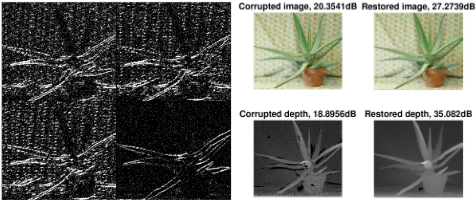
A quantitative comparison of depth channel interpolation task is shown in Figure 5. In general, GP-FA is marginally better than GP-SBN-FA, as in about 75% images GP-FA performs slightly better than GP-SBN-FA. However, GP-SBNFA is approximately 25% faster than GP-FA. GP-FA and GP-SBN-FA are consistently better than dHBP and BPFA in all images. Our approach also outperformed 5 methods described in Lu et al. (2014) (JBF, NLM, SGF, SHF, GIF). Low-Rank Matrix Completion, also in Lu et al. (2014), performs in average 0.5dB better than our methods, as that theirs is specifically designed for depth channel interpolation.
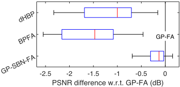
Provided that the original implementation of dHBP only applies to 2-D spatial filters, we performed another experiment on dHBP, where channel information was excluded from the covariance function, i.e., we removed k(c) m from their smoothing function. We verified that resulting PSNRs with and without channel information are about the same.
One key observation about our approach is that by removing the third covariance function, k(c) m , the resulting average PSNR decreases by about 0▷5 dB. This suggests that imputation on the depth channel can effectively borrow information from color channels via the GP prior. Another phenomenon is that for cases where the local smoothness assumption about the data does not hold, FA-GP and dHBP do not perform well. We also noticed that FA-GP yields good imputation results particularly when the image has repeated patterns. This may be explained by the fact that GPs can capture periodic behaviors, whereas smoothing kernel functions decaying over distance are likely to fail. We also found that the binary activation patterns of RGB channels are similar to each other, while the activate dictionary elements in the depth channel exhibit weaker similarities with color channels.
6 Conclusion
We have presented a dictionary learning model that captures spatial correlation of dictionary activation patterns in a principled way. Binary activation vectors indicating the presence or absence of each dictionary element are established either via a Gaussian process field followed by logistic link functions, or a Gaussian process field followed by an SBN; the SBN provides computational acceleration, and often better results. P´olya-gamma augmentation and Kronecker methods are employed for efficient MCMC inference. Experiments on realworld images demonstrated that our approach outperforms related Bayesian dictionary learning models for inpainting, denoising and depth restoration tasks.
Acknowledgements
This research was supported in part by NSF, ARO, DARPA, DOE, NGA and ONR.
@inproceedings{ijcai2016p337,
  title     = {Bayesian Dictionary Learning with Gaussian Processes and Sigmoid Belief Networks},
  author    = {Zhang, Yizhe and Henao, Ricardo and Li, Chunyuan and Carin, Lawrence},
  booktitle = {Proceedings of the Twenty-Fifth International Joint Conference on
               Artificial Intelligence, {IJCAI-16}},
  publisher = {AAAI Press / International Joint Conferences on Artificial Intelligence},
  editor    = {Subbarao Kambhampati},
  pages     = {2364--2369},
  year      = {2016},
  month     = {7},
  url       = {https://ijcai.org/proceedings/2016/337},
}
TY - CPAPER TI - Bayesian Dictionary Learning with Gaussian Processes and Sigmoid Belief Networks AU - Zhang, Yizhe AU - Henao, Ricardo AU - Li, Chunyuan AU - Carin, Lawrence T2 - Proceedings of the Twenty-Fifth International Joint Conference on Artificial Intelligence, IJCAI-16 PB - AAAI Press / International Joint Conferences on Artificial Intelligence PY - 2016 SP - 2364 EP - 2369 UR - https://ijcai.org/proceedings/2016/337 ER -Copied
Machine-readable versions of this paper, for tools and AI agents:





