
Denoising and Completion of 3D Data via Multidimensional Dictionary Learning
Proceedings of the Twenty-Fifth International Joint Conference on Artificial Intelligence. Pages 2371-2376.
Abstract
In this paper a new dictionary learning algorithm for multidimensional data is proposed. Unlike most conventional dictionary learning methods which are derived for dealing with vectors or matrices, our algorithm, named K-TSVD, learns a multidimensional dictionary directly via a novel algebraic approach for tensor factorization as proposed in [Braman, 2010; Kilmer et al., 2011; Kilmer and Martin, 2011]. Using this approach one can define a tensor-SVD and we propose to extend K-SVD algorithm used for 1-D data to a K-TSVD algorithm for handling 2-D and 3-D data. Our algorithm, based on the idea of sparse coding (using group-sparsity over multidimensional coefficient vectors), alternates between estimating a compact representation and dictionary learning. We analyze our K-TSVD algorithm and demonstrate its result on video completion and video/multispectral image denoising.
- [Aharon et al., 2006] M. Aharon, M. Elad, and A. Bruckstein. Svdd: An algorithm for designing overcomplete dictionaries for sparse representation. Trans. Sig. Proc., 54(11):4311- 4322, November 2006.
- [Boyd et al., 2011] Stephen Boyd, Neal Parikh, Eric Chu, Borja Peleato, and Jonathan Eckstein. Distributed optimization and statistical learning via the alternating direction method of mul- tipliers. Found. Trends Mach. Learn., 3(1):1-122, January 2011.
- [Braman, 2010] Karen Braman. Third-order tensors as linear op- erators on a space of matrices. Linear Algebra and its Appli- cations, pages 1241-1253, 2010.
- [Dabov et al., 2007] Kostadin Dabov, Alessandro Foi, Vladimir Katkovnik, and Karen Egiazarian. Image denoising by sparse 3d transform-domain collaborative filtering. IEEE TRANS. IMAGE PROCESS, 16(8):2080, 2007.
- [Duan et al., 2012] Guifang Duan, Hongcui Wang, Zhenyu Liu, Junping Deng, and Yen-Wei Chen. K-CPD: learning of over- complete dictionaries for tensor sparse coding. In Proceedings of the 21st International Conference on Pattern Recognition, ICPR 2012, Tsukuba, Japan, November 11-15, 2012, pages 493-496, 2012.
- [Elad and Aharon, 2006] M. Elad and M. Aharon. Image de- noising via sparse and redundant representations over learned dictionaries. Trans. Img. Proc., 15(12):3736-3745, December 2006.
- [Engan et al., 2000] Kjersti Engan, Sven Ole Aase, and John Hkon Husy. Multi-frame compression: theory and de- sign. Signal Processing, 80(10):2121-2140, 2000.
- [Fu et al., 2014] Yifan Fu, Junbin Gao, Yanfeng Sun, and Xia Hong. Joint multiple dictionary learning for tensor sparse cod- ing. In 2014 International Joint Conference on Neural Net- works, IJCNN 2014, Beijing, China, July 6-11, 2014, pages 2957-2964, 2014.
- [Goyette et al., 2012] Nil Goyette, Pierre-Marc Jodoin, Fatih Porikli, Janusz Konrad, and Prakash Ishwar. Changedetec- tion.net: A new change detection benchmark dataset. In CVPR Workshops, pages 1-8. IEEE, 2012.
- [Harshman, 1970] R. A. Harshman. Foundations of the PARAFAC procedure: Models and conditions for an" explana- tory" multi-modal factor analysis. UCLA Working Papers in Phonetics, 16(1):84, 1970.
- [Huang and Anandkumar, 2015] Furong Huang and Animashree Anandkumar. Convolutional dictionary learning through ten- sor factorization. CoRR, abs/1506.03509, 2015.
- [Kilmer and Martin, 2011] Misha E. Kilmer and Carla D. Mar- tin. Factorization strategies for third-order tensors. Linear Algebra and its Applications, 435(3):641 -658, 2011. Special Issue: Dedication to Pete Stewart on the occasion of his 70th birthday. [Kilmer et al., 2011]
- M. Kilmer, K. Braman, and N. Hao. Third order tensors as operators on matrices: A theoretical and com- putational framework. Tufts University, Department of Com- puter Science, Tech. Rep., January 2011.
- [Liu et al., 2012] Xuefeng Liu, Salah Bourennane, and Caro- line Fossati. Denoising of hyperspectral images using the PARAFAC model and statistical performance analysis. IEEE T. Geoscience and Remote Sensing, 50(10):3717-3724, 2012.
- [Peng et al., 2014] Yi Peng, Deyu Meng, Zongben Xu, Chen- qiang Gao, Yi Yang, and Biao Zhang. Decomposable nonlocal tensor dictionary learning for multispectral image denoising. In Proceedings of the 2014 IEEE Conference on Computer Vi- sion and Pattern Recognition, CVPR '14, pages 2949-2956, Washington, DC, USA, 2014. IEEE Computer Society.
- [Ramirez et al., 2010] I.
- Ramirez, P. Sprechmann, and G. Sapiro. Classification and clustering via dictionary learning with structured incoherence and shared features. In Computer Vi- sion and Pattern Recognition (CVPR), 2010 IEEE Conference on, pages 3501-3508, June 2010.
- [Renard et al., 2008] Nadine Renard, Salah Bourennane, and Jacques Blanc-Talon. Denoising and dimensionality reduc- tion using multilinear tools for hyperspectral images. In IEEE Trans. Geoscience and Remote Sensing, 2008.
- [Rubinstein et al., 2008] Ron Rubinstein, Michael Zibulevsky, and Michael Elad. Efficient implementation of the k-svd al- gorithm using batch orthogonal matching pursuit, 2008.
- [Soltani et al., 2015] Sara Soltani, Misha Elena Kilmer, and Per Christian Hansen. A tensor-based dictionary learn- ing approach to tomographic image reconstruction. CoRR, abs/1506.04954, 2015.
- [Tucker, 1966c] L. R. Tucker. Some mathematical notes on three-mode factor analysis. Psychometrika, 31:279-311, 1966c.
- [Yang et al., 2012] Jianchao Yang, Zhaowen Wang, Zhe Lin, S. Cohen, and T. Huang. Coupled dictionary training for im- age super-resolution. Image Processing, IEEE Transactions on, 21(8):3467-3478, Aug 2012.
- [Zhang and Li, 2010] Qiang Zhang and Baoxin Li. Discrimi- native k-svd for dictionary learning in face recognition. In CVPR, pages 2691-2698. IEEE Computer Society, 2010.
- [Zhang et al., 2014] Zemin Zhang, Gregory Ely, Shuchin Aeron, Ning Hao, and Misha Elena Kilmer. Novel methods for mul- tilinear data completion and de-noising based on tensor-svd. In 2014 IEEE Conference on Computer Vision and Pattern Recognition, CVPR 2014, Columbus, OH, USA, June 23-28, 2014, pages 3842-3849, 2014.
- [Zubair and Wang, 2013] S. Zubair and Wenwu Wang. Tensor dictionary learning with sparse tucker decomposition. In Dig- ital Signal Processing (DSP), 2013 18th International Confer- ence on, pages 1-6, July 2013.
References were extracted automatically from the PDF and may contain errors.
Full text extracted automatically from the PDF; figures, tables and equations may differ. The PDF is the version of record.
1 Introduction
Sparsity driven signal processing has been widely used in many areas across computer vision and image analysis, such as image restoration and classification [Aharon et al., 2006; Yang et al., 2012; Ramirez et al., 2010]. The main principle driving the gains is the idea of sparse coding, i.e. the underlying signal is compactly represented by a few large coefficients in the overcomplete dictionary, while the noise and the sampling process are incohrent. Since the performance heavily relies on the chosen dictionary, a lot of dictionary learning algorithms are developed to obtain dictionaries that are more adapted to the signal than the predefined ones, such as wavelet and DCT. In [Aharon et al., 2006], Aharon et al. proposed an algorithm called K-SVD, which efficiently learns an overcomplete dictionary from a set of training signals. The method of optimal directions (MOD)[Engan et al., 2000] shares the same effective sparse coding principle for dictionary learning as K-SVD. Discriminative K-SVD algorithm (D-KSVD) proposed in [Zhang and Li, 2010] improved the K-SVD method by unifying the dictionary and classifier learning processes. [Rubinstein et al., 2008] efficiently accelerated the K-SVD algorithm and reduced its memory consumption using a batch orthogonal matching pursuit method.
When the signal is not limited to two dimensional signals, traditional methods generally embed the high dimensional data into a vector space by vectorizing the data points; therefore the conventional matrix based approaches can still be used. This kind of vectorization, however, will break the original multidimensional structure of the signal and reduce the reliability of post processing. To this end, some dictionary learning techniques have been explored based on different tensor decompositions such as CP decomposition [Duan et al., 2012; Huang and Anandkumar, 2015], Tukcer Decomposition[Zubair and Wang, 2013; Peng et al., 2014; Fu et al., 2014] and tensor-SVD[Soltani et al., 2015]. In [Duan et al., 2012], the authors developed an algorithm called K-CPD which learns high order dictionaries based on the CP decomposition. [Zubair and Wang, 2013] proposed a tensor dictionary learning algorithm based on the Tucker model with sparsity constraints over its core tensor, and applied gradient descent algorithm to learn overcomplete dictionaries along each mode of the tensor (see [Tucker, 1966c] for definition of tensor modes). Peng et al. [Peng et al., 2014] presented a tensor dictionary learning algorithm based on Tucker model with Group-block-sparsity constraint on the core tensor with good performance.
In this paper, we present a novel multidimensional dictionary learning approach based on a notion of tensor-SVD proposed in [Braman, 2010; Kilmer et al., 2011; Kilmer and Martin, 2011]. Essentially the t-SVD is based on an operator theoretic interpretation of the 3rd order tensors [Braman, 2010], as linear operators over the set of 2-D matrices. This framework has recently been used for dictionary learning for 2-D images in [Soltani et al., 2015], but the authors there employ a different algorithm and the problem considered is tomographic image reconstruction. Moreover we will also consider the problem of filling in missing data by sparse coding using the learned dictionary.
The paper is organized as follows. In section 2 we go over the definitions and notations, then illustrate the main differences and advantages over other tensor decomposition methods. Section 3 formulates the objective function for tensor dictionary learning problem using t-SVD, by introducing the "tubal sparsity" of third-order tensors. Our tensor dictionary learning model and detailed algorithm to solve the problem are presented in Section 4. In Section 5 we show experiment results on third order tensor completion and denoising. Finally we conclude our paper in Section 6.
2 Brief Overview of T-SVD Framework
2.1 Notations and Preliminaries
In this part we briefly describe the notations used throughout the paper, and the t-SVD structure proposed in [Braman, 2010; Kilmer and Martin, 2011; Kilmer et al., 2011].
A tensor is a multidimensional array of numbers. For example, vectors are first order tensors, matrices are second order tensors. Tensors of size n1⇥n2⇥n3 are called third order tensors. In this paper, third order tensors are represented in bold script font A.
A Slice of an n-th order tensor is a 2-D section defined by fixing all but two indices. For a third order tensor A, we will use the Matlab notation A(k↪ :↪ :) , A(:↪ k↪ :) and A(:↪ :↪ k) to denote the k-th horizontal, lateral and frontal slices. A(k) is particularly used to represent A(:↪ :↪ k), and -!Ak represents A(:↪ k↪ :). We also call such -!Ak tensor columns.
A Fiber (or Tube) is a 1-D section obtained by fixing all indices but one. For a third order tensor, A(:↪ i↪ j), A(i↪ :↪ j) and A(i↪ j↪ :) denote the (i↪ j)-th mode-1, mode-2 and mode3 fiber. Specifically we let ~a 2 R1⇥1⇥n3 denote an n3-tube.
The approach in [Braman, 2010; Kilmer et al., 2011; Kilmer and Martin, 2011] rests on defining a multiplication operation, referred to as the tensor-product (t-product) between two third order tensors. This is done by using a commutative operation, in particular circular convolution between tensor tubes as defined below.
Definition 2.1.1. (t-product) The t-product between A 2 Rn1⇥n2⇥n3 and B 2 Rn2⇥n4⇥n3 is an n1 ⇥n4 ⇥n3 tensor C whose (i↪ j)-th tube C(i↪ j↪ :) is given by
where i = 1↪ 2↪ ▷▷▷↪ n1, j = 1↪ 2↪ ▷▷▷↪ n4. When a third order tensor is viewed as a matrix of tubes along the third dimension, the t-product is analogous to the matrix multiplication except that the multiplication between numbers are replaced by the circular convolution between tubes.
Remark 2.1.1. From the relationship between circular convolution and Discrete Fourier Transform(DFT), the t-product of A and B can be computed efficiently in Fourier domain. Specifically, let bA = fft(A↪ [ ]↪ 3) and bB = fft(B↪ [ ]↪ 3) be the tensors obtained by taking the Fast Fourier Transform (FFT) along the tube fibers in third dimension of A and B, then we can compute the t-product of A and B through the following,
C = ifft(bC↪ [ ]↪ 3) Definition 2.1.2. (Tensor transpose) The conjugate transpose of a tensor A 2 Rn1⇥n2⇥n3 is an n2 ⇥ n1 ⇥ n3 tensor AT obtained by taking the conjugate transpose of each frontal slice of A, then reversing the order of transposed frontal slices 2 through n3.
Definition 2.1.3. (Identity tensor) The identity tensor I 2 Rn⇥n⇥n3 is defined as follows,
where In⇥n is the identity matrix of size n ⇥ n.
Definition 2.1.4. (Orthogonal Tensor) A tensor Q 2 Rn⇥n⇥n3 is orthogonal if it satisfies
Definition 2.1.5. (f-diagonal Tensor) A tensor is called f-diagonal if each frontal slice of this tensor is a diagonal matrix.
2.2 Tensor Singular Value Decomposition(t-SVD)
We now define the tensor Singular Value Decomposition using the t-product introduced in previous section.
Definition 2.2.1. The t-SVD of a third-order tensor M 2 Rn1⇥n2⇥n3 is given by
where ⇤ denotes the t-product, U 2 Rn1⇥n1⇥n3 and V 2 Rn2⇥n2⇥n3 are orthogonal tensors. S 2 Rn1⇥n2⇥n3 is a rectangular f-diagonal tensor.
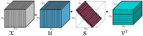
Figure 1 illustrates the t-SVD of 3rd order tensors. Similar to the t-product, we can also compute t-SVD in Fourier domain, see Algorithm 1.
Algorithm 1 T-SVD of third order tensors
Input: M2 Rn1⇥n2⇥n3 Output: U 2 Rn1⇥n1⇥n3 , V 2 Rn2⇥n2⇥n3 and S 2 Rn1⇥n2⇥n3 such that M= U⇤ S ⇤ VT. cM= ↵t(M↪ [ ]↪ 3); for i = 1 to n3 do [U↪ S↪ V] = SVD(cM(:↪ :↪ i)) bU(:↪ :↪ i) =U; bS(:↪ :↪ i) = S; bV(:↪ :↪ i) =V; end for U = i↵t(bU↪ [ ]↪ 3), S = i↵t(bS↪ [ ]↪ 3), V = i↵t(bV↪ [ ]↪ 3).As discussed in [Zhang et al., 2014], t-SVD has many advantages over the classical tensor decompositions such as CANDECOMP/PARAFAC[Harshman, 1970] and Tucker[Tucker, 1966c]. For example, given a fixed rank, the computation of CANDECOMP/PARAFAC decomposition can be numerically unstable, since calculating the rank-1 components in this model is difficult. Similarly, finding the best Tucker multi-rank ~r approximation to a tensor is numerically expensive and often does not yield the best fit to the original tensor. However, the computation of t-SVD is very easy since one only needs to do several SVDs as shown in Algorithm 1. Another very important property is the optimality approximation of t-SVD [Kilmer and Martin, 2011], described in the following.
Theorem 2.2.1. Let M = U ⇤ S ⇤ VT be the t-SVD of M 2 Rn1⇥n2⇥n3 . Then for k < min(n1↪ n2), define Mk = Pki=1 U(:↪ i↪ :) ⇤ S(i↪ i↪ :) ⇤ V(:↪ i↪ :)T, we have
where M = ¶X ⇤ Y♣X 2 Rn1⇥k⇥n3 ↪ Y 2 Rk⇥n2⇥n3 ♦.
If we define tensor tubal rank of M to be the number of non-zero diagonal tubes in S[Zhang et al., 2014], then this theorem is saying that Mk is the closest tensor toM in Frobenius norm among all tensors of tensor tubal rank at most k.
2.3 t-linear Combination of Tensor Dictionaries and Coefficients
As in the matrix case, given an overcomplete dictionary D 2 Rn⇥K which contains K prototype signal-atoms for columns, a signal y 2 Rn can be represented as a linear combination of columns of D
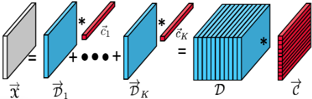
where x 2 RK is called the representation coefficient vector of y. This set up could be easily extended to 3rd order tensors using the framework outlined in the previous section. Given K tensor columns (or dictionary atoms) -!Dk 2 Rn1⇥1⇥n3 , we represent a tensor signal -!X 2 Rn1⇥1⇥n3 using the t-linear combination of the given tensor dictionaries as follows,
where ¶~ck♦Kk=1 are tubes of size 1 ⇥ 1 ⇥ n3; -!C 2 RK⇥1⇥n3 is called coefficient tensor obtained by aligning all the ~ck. D = ¶-!D1↪ -!D2↪ ▷▷▷↪ -!DK♦ 2 Rn1⇥K⇥n3 is the tensor dictionary. The representation (6) may either be exact or approximate satisfying
for some ✏ > 0. When K > n, we say the tensor dictionary D is overcomplete.
3 ProblemFormulation
In this section, we introduce our tensor dictionary learning model and the related algorithm.
3.1 FromMatrix to Tensor Dictionary Learning
Given an overcomplete dictionary D 2 Rn⇥K with K > n, if D is full rank, there are infinite number of solutions to the representation problem (5); therefore in order to constran the solution set, one common approach is to enforce sparsity. As in classic dictionary learning model which was first designed for the purpose of reconstruction, one adaptively learns an overcomplete dictionary using the training data, which leads to the best possible representation of the data with sparsity constraints. Specifically, given training data ¶yi♦ni=1 2 Rd where d is the dimensionality and n is the total number of training data used, dictionary learning methods aim at finding an overcomplete dictionary D 2 Rd⇥K with K > d, and a coefficient matrix X = [x1↪ x2↪ ▷▷▷↪ xn] 2 RK⇥n by the following optimization problem,
where k · kq↪ q ≥ 1 is the `q norm which represents different sparsity regularization.
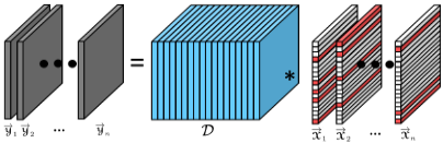
Using t-SVD structure discussed in the previous section, we generalize this dictionary learning model to higher dimensional cases. Given training data as tensor columns ¶-!Yi♦ni=1 2 Rd⇥1⇥n3 , we want to find a dictionary D 2 Rn⇥K⇥n3 with K > n, and "tubal sparse" tensor coefficients ¶-!Xi♦ni=1 2 RK⇥1⇥n3 to represent the training data using t-product. The tubal sparsity of a tensor column is defined in [Zhang et al., 2014] as follows.
Definition 3.1.1. (tensor tubal sparsity) Given a tensor column -!X, the tensor tubal sparsity k · kTS is defined as the number of non-zero tubes of -!X in the third dimension.
Then we can construct our dictionary learning model:
or equivalently,
where Y = h-!Y1↪ -!Y2↪ ▷▷▷↪ -!Yn i 2 Rd⇥n⇥n3 and X = h-!X1↪ -!X2↪ ▷▷▷↪ -!Xn i 2 RK⇥n⇥n3 . Figure 3 illustrates the tensor sparse coding model. Note that if the jth tube of -!Xi(j↪ 1↪ : ) is zero, then it means that the jth dictionary D(:↪ j↪ :) is not being used in the representation of -!Y i.
3.2 K-TSVD
We now discuss our tensor dictionary learning model in details. Our model is called K-TSVD since it is a general extension from classic K-SVD to high dimensional tensor based on t-SVD. Similarly to K-SVD algorithm, K-TSVD also consists of two stages: the tensor sparse coding stage and the tensor dictionary update stage. First let's consider the sparse coding stage where the tensor dictionary D is fixed. So we need to solve
subject to kXkTS T0
or alternatively we can work on an equivalent form,
for some positive λ. Since the sparsity measure is computational intractable in both matrix and tensor cases, we use the k · k1↪1↪2 norm [Zhang et al., 2014] instead as a convex relaxation for the tubal sparsity, where the k · k1↪1↪2 norm of a 3rd order tensor X is defined as
If we regard a third dimensional tube ~x 2 R1⇥1⇥n3 as a n3⇥1 column vector, then the `1↪1↪2 norm of X is just the summation of `2 norm of all such tubes along the third dimension in X.
Replacing the tubal sparsity with the `1↪1↪2 norm, the problem becomes
In order to solve this problem, one more definition is needed here. For a third order tensor A 2 Rn1⇥n2⇥n3 , define the block diagonal form A in Fourier domain as follows,
bA(n3) where bA = fft(A↪ [ ]↪ 3) and A(i) is the ith frontal slice of A. Then (13) can be equivalently reformulated in Fourier domain as
where the pn3 factor comes from the fact that kXkF = kbXkF◁pn3 [Zhang et al., 2014]. Use the general framework of Alternating Direction Method of Multipliers (ADMM) [Boyd et al., 2011], we can solve this optimization problem recursively with the following algorithm:
where ⇢ > 0. (15) is essentially a least square minimization problem and we can separately solve it in each frontal slice of bX (or equivalently, each diagonal block of X). Let Ck+1 = Xk+1 +Qk◁⇢, the update of (16) is given by
where (·)+ = max(0↪ ·).
The second stage of our tensor dictionary learning model is dictionary update. Given fixed D and X, suppose we only want to update the k-th element of D, we can decompose the error term as follows,
Ek here stands for the representation error when the k-th atom D(:↪ k↪ :) is removed from the dictionary. The next step is to find D(:↪ k↪ :)⇤X(k↪ :↪ :) which best approximates Ek, so that the error term is minimized. This is essentially to compute the best tubal rank-1 approximation using Theorem 2.2.1. Since we need to maintain the tubal sparsity of X and don't want to fully fill X(k↪ :↪ :), let wk = ¶i♣X(k↪ i↪ :) 6= 0↪ i = 1↪ 2↪ ▷▷▷↪ n♦ be the set of indices where data Y uses tensor dictionary D(:↪ k↪ :) and restrict Ek by choosing the tensor columns corresponding to wk to obtain Rk : R(:↪ i↪ :) = E(:↪wk(i)↪ : )↪ i = 1↪ 2↪ ▷▷▷↪ ♣wk♣. From Theorem 2.2.1, we apply t-SVD on Rk to get U↪ S and V, and take the first tensor column of U to update D(:↪ k↪ :), use S(1↪ 1↪ :) ⇤ V(:↪ 1↪ :)T to renovate the coefficient tensors which use the k-th dictionary. To accelerate the algorithm we only compute the approximate rank-1 SVDs in Fourier domain when we compute t-SVD of R. The complete algorithm is presented in Algorithm 2. Note that the optimization problem in Step 1 is convex and we use ADMM [Boyd et al., 2011] with global convergence guarantees. Similarly to K-SVD, the dictionary update stage is only guaranteed to converge to a local minimum theoretically. However, in practice the output dictionary of K-TSVD performs very well as we will see in the next section.
Algorithm 2 K-TSVD
Input : Observed tensor data Y = ¶-!Yi♦n2 i=1 2 Rn1⇥n2⇥n3 , λ > 0.
Initialize: Dictionary D0 2 Rn1⇥K⇥n3
Repeat until convergence:
- 1: Compute the sparse coefficient tensor using (15)-(17):
- 2: for k = 1↪ 2↪ ▷▷▷↪K do
- 3: Let wk = ¶i♣X(k↪ i↪ :) 6= 0♦ be the set of indices where data Y uses dictionary D(:↪ k↪ :).
- 4: ComputeEk = Y-Pj6=k D(:↪ j↪ :)⇤X(j↪ :↪ :)T, which is the over all error without using the k-th dictionary atom D(:↪ k↪ :).
- 5: Restrict Ek by choosing only the tensor columns corresponding to wk and obtain Rk:
for i = 1↪ 2↪ ▷▷▷↪ ♣wk♣.
- 6: Compute the t-SVD of Rk:
- 7: Update D(:↪ k↪ :) = U(:↪ 1↪ :).
- 8: Update X(k↪wk↪ :) = S(1↪ 1↪ :) ⇤ V(:↪ 1↪ :)T.
- 9: end for
Output: Trained tensor dictionary D.
4 Experiment Results
4.1 FillingMissing Pixels in Tensors
In this section we consider the application of filling missing pixels in third order tensors. Suppose that we are given a video with dead pixels, where the dead pixels mean pixel values are deleted or missing on some fixed positions of each frame. Specifically, let ⌦ indicate the set of indices of the remaining pixels andMbe the data tensor, thenM(i↪ j↪ :) = 0 for all (i↪ j) ◁2 ⌦. Our goal is to recover such tensors with missing pixels. Suppose D is the learned overcomplete dictionary on the training data, define P⌦ as an orthogonal projector such that P⌦(M)(i↪ j↪ :) =M(i↪ j↪ :), if (i↪ j) 2 ⌦ and 0 otherwise. Then for each patch -!Mk in the test data, the reconstruction of this patch is D⇤-!C k, where -!C k is the solution to
which can be solved in the same manner as (13).
We utilized a basketball video here to apply K-TSVD algorithm and reconstruct M from missing pixels. There are 40 frames in the video and the resolution of each frame is 144 ⇥ 256. To learn the overcomplete dictionary using KTSVD, we randomly took 9000 overlapping block patches of size 8⇥8⇥10 from the first 30 frames, saved them as tensor columns of size 64 ⇥ 1 ⇥ 10, and obtained our training data Y of total size 64 ⇥ 9000 ⇥ 10. All these patches were used to train a tensor dictionary with K = 256 atoms. The last 10 frames of the video were used for testing. We took the total 576 disjoint 8⇥8⇥10 blocks in the last 10 frames, saved each block into a tensor column, and obtained our training data of size 64 ⇥ 576 ⇥ 10.
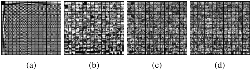
We investigated the performance of K-TSVD by comparing it with K-SVD and DCT. In K-SVD, in order to have a fair comparison, for each test frame we also randomly trained 10000 block patches of size 8⇥8 in the first 30 frames. We visualize an example of the overcomplete DCT dictioanry, the K-SVD learned dictionary and the K-TSVD learned dictionary in Figure 4. One frame with 50% and 70% missing pixels and its reconstructions are shown in Figure 5. As one can see the reconstruction based on K-TSVD learned dictionary has a better quality. Figure 5(e) shows the reconstruction error (RE) comparison of those three approaches, where the error is computed via RE = pkX-Xreck2F ◁N, N is the total number of pixels in the data. We can see that when the percentage of missing pixels is small, all three methods perform equally well. With more missing pixels, K-TSVD gives better performance over the other two methods.
4.2 Multispectral Image and Video Denoising
In order to further test the proposed method, we applied our algorithm on multispectral/hyperspectral images and video data denoising. In the first experiment the multispectral data was from the Columbia datasets 1 , each dataset contains 31 real-world images of size 512 ⇥ 512 and is collected from 400nm to 700nm at 10nm steps. In our experiment we resized each image into size of 205 ⇥ 205, and took images of the last 10 bands to accelerate the speed of training tensor dictionaries. Therefore the total size of the tensor data we used here is 205 ⇥ 205 ⇥ 10. Further work is required to fully deploy the algorithm in large-scale high order tensor
1 http://www1.cs.columbia.edu/CAVE/databases/multispectral/
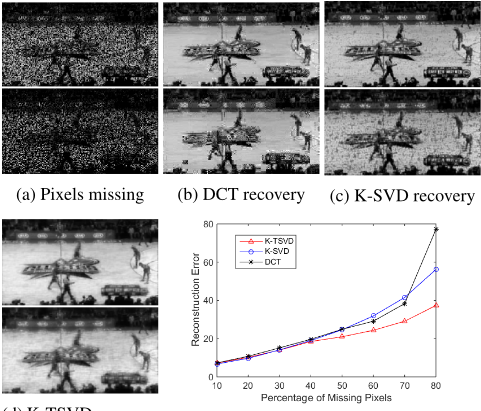
(d) K-TSVD recovery (e) Reconstruction error comparison.
Figure 5: The reconstruction result frommissing pixels on the basketball video. The different rows are for 50% and 70% of missing pixels respectively.
applications.
For the noise model we consider the fixed-location defects without knowing the noisy positions, which commonly exists in video and multispectral images. On image of each bandwidth, some fixed pixel locations are corrupted with very high noise and our task is to recover the image. Specifically in our experiment we picked a sparse number of pixel locations and added Gaussian noise on these positions of each image. Let ⌦ indicate the set of noisy pixel locations, then what we did was for each (i↪ j) 2 ⌦, k = 1↪ 2↪ ▷▷▷↪ 10, Y(i↪ j↪ k) = Y(i↪ j↪ k) + wijk, where Y is the clean tensor and wijk ⇠ N(0↪ σ) is the additive Gaussian noise.
To train the data and learn the dictionaries, similarly to what we did in the previous experiment, we randomly took 10000 overlapping patches of size 8 ⇥ 8 ⇥ 10 from the noisy tensor data, which is about a quarter of all the overlapping patches in the data. For a fair comparison, in K-SVD we also randomly select 10000 overlapping patches of size 8⇥8 within each noisy image.
| Sparsity Noise level | 5% 100 | 10% 100 | 15% 100 | 10% 150 | 10% 200 |
|---|---|---|---|---|---|
| Noisy image | 20.96 | 18.18 | 16.35 | 14.75 | 12.10 |
| K-SVD | 22.73 | 22.60 | 22.49 | 22.38 | 22.00 |
| 3DK-SVD | 22.61 | 22.53 | 22.47 | 22.41 | 22.20 |
| BM3D | 26.95 | 26.62 | 26.36 | 25.23 | 24.29 |
| LRTA | 23.54 | 26.84 | 26.65 | 23.90 | 22.03 |
| DNMDL | 24.07 | 23.73 | 25.16 | 17.89 | 16.83 |
| PARAFAC | 27.07 | 26.86 | 26.72 | 26.13 | 25.24 |
| KTSVD | 27.19 | 26.98 | 26.79 | 26.18 | 25.44 |
The denoising process of our method includes a tensor sparse coding stage based on the learned tensor dictionary. We extracted each 8⇥8⇥10 patch in the noisy multispectral images and solved the tensor sparse coding problem (13) to obtain the denoised patch. Following a similar idea in [Elad and Aharon, 2006], we averaged all the denoised patches with some relaxation obtained by averaging with the original noisy data then got our denoised tensor.
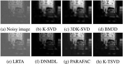
To test the performance of our method, we compared our K-TSVD to these methods: K-SVD (band-wise)[Aharon et al., 2006; Elad and Aharon, 2006] 3D K-SVD [Elad and Aharon, 2006], BM3D (band-wise) [Dabov et al., 2007], LRTA[Renard et al., 2008], DNMDL[Peng et al., 2014] and PARAFAC[Liu et al., 2012]. The result with σ = 100 and the sparsity of noisy pixels equaling 10% is shown in Figure 6. The detailed PSNR comparison on different noise levels of these methods is in Table 1. We can see that our algorithm has a better performance over the other competing methods on most cases.
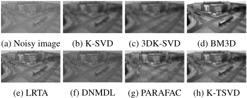
We also applied K-TSVD algorithm on video denoising. The video that we used here was footage from a still camera view of a traffic intersection [Goyette et al., 2012]. The resolution of each frame is 175 ⇥ 328, and we performed our method on every 10 frames. Figure 7 shows one frame of the denoising result with sparsity = 10% and noise level 100. As one can see in this experiment K-TSVD perform very well.
5 Conclusion
In this paper, we present a new method for tensor dictionary learning algorithm K-TSVD, using the t-SVD framework. Our main contribution lies in explicitly integrating the sparse coding of third order tensors in t-SVD sense, and based on this we generalize the K-SVD dictionary learning model to deal with higher order tensors. The experimental results show that our approach yields very good performance on video completion and multispectral images denoising.
6 Acknowledgements
This work was supported in part by the National Science Foundation (NSF) grant CCF:1319653.
@inproceedings{ijcai2016p338,
  title     = {Denoising and Completion of 3D Data via Multidimensional Dictionary Learning},
  author    = {Zhang, Zemin and Aeron, Shuchin},
  booktitle = {Proceedings of the Twenty-Fifth International Joint Conference on
               Artificial Intelligence, {IJCAI-16}},
  publisher = {AAAI Press / International Joint Conferences on Artificial Intelligence},
  editor    = {Subbarao Kambhampati},
  pages     = {2371--2376},
  year      = {2016},
  month     = {7},
  url       = {https://ijcai.org/proceedings/2016/338},
}
TY - CPAPER TI - Denoising and Completion of 3D Data via Multidimensional Dictionary Learning AU - Zhang, Zemin AU - Aeron, Shuchin T2 - Proceedings of the Twenty-Fifth International Joint Conference on Artificial Intelligence, IJCAI-16 PB - AAAI Press / International Joint Conferences on Artificial Intelligence PY - 2016 SP - 2371 EP - 2376 UR - https://ijcai.org/proceedings/2016/338 ER -Copied
Machine-readable versions of this paper, for tools and AI agents:





