
Learning Cross-View Binary Identities for Fast Person Re-Identification
Proceedings of the Twenty-Fifth International Joint Conference on Artificial Intelligence. Pages 2399-2405.
Abstract
In this paper, we propose to learn cross-view binary identities (CBI) for fast person re-identification. To achieve this, two sets of discriminative hash functions for two different views are learned by simultaneously minimising their distance in the Hamming space, and maximising the cross-covariance and margin. Thus, similar binary codes can be found for images of a same person captured at different views by embedding the images into the Hamming space. Therefore, person re-identification can be solved by efficiently computing and ranking the Hamming distances between the images. Extensive experiments are conducted on two public datasets and CBI produces comparable results as state-ofthe- art re-identification approaches but is at least 2200 times faster.
- [Ahmed et al., 2015] Ejaz Ahmed, Michael Jones, and Tim K. Marks. An improved deep learning architecture for person re-identification. In Proc. CVPR, 2015.
- [Bronstein and Bronstein, 2010] Michael M. Bronstein and Alexander M. Bronstein. Data fusion through cross- modality metric learning using similarity-sensitive hash- ing. In Proc. CVPR, 2010.
- [Chen et al., 2015] Dapeng Chen, Zejian Yuan, Gang Hua, Nanning Zheng, and Jingdong Wang. Similarity learning on an explicit polynomial kernel feature map for person re-identification. In Proc. CVPR, 2015.
- [Cheng et al., 2011] Dong Seon Cheng, Marco Cristani, Michele Stoppa, Loris Bazzani, and Vittorio Murino. Cus- tom pictorial structures for re-identification. In Proc. BMVC, 2011.
- [Cortes and Vapnik, 1995] Corinna Cortes and Vladimir Vapnik. Support-vector networks. Machine Learning, 20:273-297, 1995.
- [Ding et al., 2014] Guiguang Ding, Yuchen Guo, and Jile Zhou. Collective matrix factorization hashing for multi- modal data. In Proc. CVPR, 2014.
- [Farenzena et al., 2010] M. Farenzena, L. Bazzani, A. Pe- rina, V. Murino, and M. Cristani. Person re-identification by symmetry-driven accumulation of local features. In Proc. CVPR, 2010.
- [Gong and Lazebnik, 2011] Yunchao Gong and Svetlana Lazebnik. Iterative quantization: A procrustean approach to learning binary codes. In Proc. CVPR, 2011.
- [Gong et al., 2013] Shaogang Gong, Marco Cristani, and Shuicheng Yan. Person Re-Identification. Advances in Computer Vision and Pattern Recognition. Springer, 2013.
- [Gray and Tao, 2008] Douglas Gray and Hai Tao. Viewpoint invariant pedestrian recognition with an ensemble of local- ized features. In Proc. ECCV, 2008.
- [Hotelling, 1936] Harold Hotelling. Relations between two sets of variates. Biometrika, 28:321-377, 1936.
- [Kostinger et al., 2012] Martin Kostinger, Martin Hirzer, Paul Wohlhart, Peter M. Roth, and Horst Bischof. Large scale metric learning from equivalence constraints. In Proc. CVPR, 2012.
- [Kumar and Udupa, 2011] Shaishav Kumar and Raghaven- dra Udupa. Learning hash functions for cross-view sim- ilarity search. In Proc. IJCAI, 2011.
- [Lampert and Kromer, 2010] Christoph H. Lampert and Oliver Kromer. Weakly-paired maximum covariance anal- ysis for multimodal dimensionality reduction and transfer learning. In Proc. ECCV, 2010.
- [Lee et al., 2006] Honglak Lee, Alexis Battle, Rajat Raina, and Andrew Y. Ng. Efficient sparse coding algorithms. In Proc. NIPS, 2006.
- [Li et al., 2014] Wei Li, Rui Zhao, Tong Xiao, and Xiaogang Wang. Deepreid: Deep filter pairing neural network for person re-identification. In Proc. CVPR, 2014.
- [Liao et al., 2015] Shengcai Liao, Yang Hu, Xiangyu Zhu, and Stan Z. Li. Person re-identification by local maximal occurrence representation and metric learning. In Proc. CVPR, 2015.
- [Long et al., 2015] Mingsheng Long, Jianmin Wang, , and Philip S. Yu. Quantized correlation hashing for fast cross- modal search. In Proc. IJCAI, 2015.
- [Loy et al., 2013] Chen Change Loy, Chunxiao Liu, and Shaogang Gong. Person re-identification by manifold ranking. In Proc. ICIP, 2013.
- [Paisitkriangkrai et al., 2015] Sakrapee Paisitkriangkrai, Chunhua Shen, and Anton van den Hengel. Learning to rank in person re-identification with metric ensembles. In Proc. CVPR, 2015.
- [Pedagadi et al., 2013] Sateesh Pedagadi, James Orwell, Sergio Velastin, and Boghos Boghossian. Local fisher dis- criminant analysis for pedestrian re-identification. In Proc. CVPR, 2013.
- [Prosser et al., 2010] Bryan Prosser, Wei-Shi Zheng, Shao- gang Gong, and Tao Xiang. Person re-identification by support vector ranking. In Proc. BMVC, 2010.
- [Rastegari et al., 2013] Mohammad Rastegari, Jonghyun Choi, Shobeir Fakhraei, Hal Daume III, and Larry S. Davis. Predictable dual-view hashing. In Proc. ICML, 2013.
- [Wang et al., 2007] Xiaogang Wang, Gianfranco Doretto, Thomas Sebastian, Jens Rittscher, and Peter Tu. Shape and appearance context modeling. In Proc. CVPR, 2007.
- [Weiss et al., 2008] Yair Weiss, Antonio Torralba, and Rob Fergus. Spectral hashing. In Proc. NIPS, 2008.
- [Yang et al., 2014] Yang Yang, Jimei Yang, Junjie Yan, Shengcai Liao, Dong Yi, and Stan Z. Li. Salient color names for person re-identification. In Proc. ECCV, 2014.
- [Zhai et al., 2013] Deming Zhai, Hong Chang, Yi Zhen, Xi- anming Liu, Xilin Chen, and Wen Gao. Parametric local multimodal hashing for cross-view similarity search. In Proc. IJCAI, 2013. IJCAI
- [Zhang et al., 2011] Dan Zhang, Fei Wang, and Luo Si. Composite hashing with multiple information sources. In Proc. SIGIR, 2011.
- [Zhao et al., 2013a] Rui Zhao, Wanli Ouyang, and Xiaogang Wang. Person re-identification by salience matching. In Proc. ICCV, 2013.
- [Zhao et al., 2013b] Rui Zhao, Wanli Ouyang, and Xiaogang Wang. Unsupervised salience learning for person re- identification. In CVPR, 2013.
- [Zhao et al., 2014] Rui Zhao, Wanli Ouyang, and Xiao- gang Wang. Learning mid-level filters for person re- identification. In CVPR, 2014.
- [Zheng et al., 2012] Wei-Shi Zheng, Shaogang Gong, and Tao Xiang. Re-identification by relative distance compar- ison. IEEE TPAMI, 2012.
References were extracted automatically from the PDF and may contain errors.
Full text extracted automatically from the PDF; figures, tables and equations may differ. The PDF is the version of record.
1 Introduction
Person re-identification addresses the problem of associating people, at different locations and times, observed by the nonoverlapping Closed-Circuit TeleVision system. It has various potential applications, such as long-term multi-person tracking, person re-acquisition and forensic search [Gong et al., 2013]. Due to the various difficulties including illumination changes, viewpoint and pose variations, inter-object occlusions and low resolution images, person re-identification is still a very challenging task and far from being tackled.
Most of the existing approaches can be categorised into two groups: learning features which are invariant to view changes [Gray and Tao, 2008; Li et al., 2014] and learning the metric functions which are used to rank the pairs of observations from different views [Prosser et al., 2010; Zheng et al., 2012; Pedagadi et al., 2013]. However, in spite of their good performance on public datasets, existing methods generally neglect considering the efficiency of the algorithm in the matching stage. In fact, the searching speed of a re-identification algorithm plays a significant role in real-world applications.
In general, the efficiency of matching mainly depends on two aspects: (1) the number of samples stored in the gallery set; (2) the definition of similarity. As for the first aspect, it is impossible to reduce the number of samples. It is because [Gong et al., 2013]: (1) A large number of surveillance cameras have been installed in public spaces assembled with hundreds of thousands of persons, even in a day. (2) Re-identification in open environments can potentially scale to arbitrary levels, covering huge spatial areas spanning not just different buildings but also different cities, or countries, leading to an overwhelming quantity of "big data". (3) Person re-identification can be extended from multi-camera networks to distributed Internet spaces. Therefore, with an explosive growth of images, speeding up the matching stage of a re-identification system by designing a more advantageous similarity criterion is an essential and non-replaceable option.
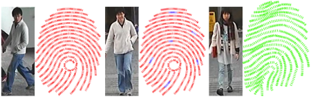
In this paper, a novel approach, learning Cross-view Binary Identities (CBI), is proposed to reduce the computational burden for person re-identification. In fact, hashing has been widely used for nearest neighbour search in computer vision areas, such as image retrieval, object recognition and image matching, but it has been seldom used in re-identification. Using the hash functions, various special properties can be preserved in the learned codes, such as locality, variance and affinity. For two observations xa and xb of one person in two different views, CBI can learn two similar codes, which are considered as the identity (ID) of that person, as shown in Fig. 1. The learned binary codes enable efficient similarity search in different views using the Hamming distance between codes. Moreover, compact binary codes are extremely economical for large-scale data storage.
Our contributions are three-fold: (1) By learning the binary codes, each person has a similar identity across different views. Due to the efficiency of binary codes, person re-identification in a huge dataset can be realised. (2) In CBI, variances of learned bits, cross-covariance and margin of learned hash codes are simultaneously maximised and an efficient iterative optimisation solution is introduced. (3) Moreover, in CBI, a theoretical proof is given to guarantee the transfer from Hamming space to Euclidean space. Unlike most methods, which directly relax the sign function, such as [Rastegari et al., 2013], we consider the theoretical reason behind when it is safe to relax the sign function.
2 RelatedWorks
To address the challenge of person re-identification, many efforts have been made along the two directions: learning discriminative features and learning the metric functions. Moreover, both aspects are considered to further improve the performance in [Liao et al., 2015].
On the one hand, the learned features are generally invariant to the view changes and simple metrics are used for matching. Various methods including local patches [Gray and Tao, 2008], colour distributions over colour names (SCNCD) [Yang et al., 2014], and salience learning [Zhao et al., 2013b] are proposed to learn discriminative features for person reidentification. In [Li et al., 2014], deep learning is exploited to automatically learn features for the re-identification task and the deep framework has been improved in [Ahmed et al., 2015] by incorporating neighbouring locations of other images.
On the other hand, complex distance metrics are learned to rank the pairs of observations from different views. Some metric learning related algorithms including Support Vector Ranking (PRSVM) [Prosser et al., 2010], relative distance comparison (PRDC) [Zheng et al., 2012], equivalence constraints [Kostinger et al., 2012] and dimensionality reduction [Pedagadi et al., 2013] to learn effective distance for person re-identification. Very recently, ensemble metrics, such as a mixture of similarities [Chen et al., 2015] and an ensemble of distances [Paisitkriangkrai et al., 2015], are exploited to discover multiple matching patterns.
Despite the promising performance achieved by the existing methods, all of them suffer from a huge computational burden in the test stage. Due to the efficient nearest neighbour search using binary codes, hashing techniques have been widely adopted in many vision applications, especially in indexing large-scale data. Composite Hashing with Multiple Information Sources (CHMIS) [Zhang et al., 2011] and the Cross View Hashing (CVH) [Kumar and Udupa, 2011] extend the SH [Weiss et al., 2008] from different aspects, respectively. The boosting algorithms are adopted to embed the input data from two arbitrary spaces into a same Hamming space by Cross-Modality Similarity Sensitive Hashing (CMSSH) [Bronstein and Bronstein, 2010]. Considering the maximum margin, Predictable Dual-view Hashing (PDH) [Rastegari et al., 2013] explores a joint formulation for learning binary codes of data from two different views. Collective Matrix Factorisation Hashing (CMFH) [Ding et al., 2014] is based on the assumption that the interlinked data should have the same latent factors and the hash codes can be learned from these factors. Moreover, local functions [Zhai et al., 2013] and correlation-maximal mappings [Long et al., 2015] are exploited to learn the common binary codes.
In this paper, we accomplish person re-identification by learning a set of hash functions for each view. From the feature learning perspective, CBI learns a discriminative binary representation for each person. Furthermore, from the metric learning perspective, a more efficient distance metric in the Hamming space is learned for matching. Moreover, most of the above hashing methods are exploited to preserve the local properties in intra-module and inter-module. However, since normally very few images for each person exist in one view, the extracted features do not meet the local smoothness assumption. Instead, CBI focuses on learning similar binary codes for a person under different views but the Hamming distances between different persons will be maximised.
3 Learning Cross-view Binary Identities
For two different camera views: a and b, we can collect two training datasets Xa = ¶x1a ↪ x2a ↪ · · · ↪ xna ♦ and Xb = ¶x1b ↪ x2b ↪ · · · ↪ xnb ♦, where xia is a column vector observed by view a for person i and n is the number of paired samples (xia ↪ xib ). Our aim is to find K hash functions F = ¶f 1 v ↪ · · · ↪ f K v ♦ for each view v 2 ¶a↪ b♦ and yv(k) = f k v (xv). In this paper, the hash functions are constructed by a set of linear hyperplanes: Wv = ¶w1 v ↪ w2 v ↪ · · · ↪wK v ♦. Thus, for dataset Xv, we obtain Yv = ¶y1 v ↪ y2 v ↪ · · · ↪ yn v ♦ by using yik v = sign((wk v )T xiv ). It is obvious that yiv 2 ¶-1↪ 1♦K . For simplicity, we can write it as: Yv = sign(W T v Xv).
For a person with an image in the probe view, the first step is to calculate the ID by using the learned projections. Next, the ID can be used to retrieve the images of persons with similar IDs in the gallery view. The IDs of persons in the gallery view can be obtained in advance. Finally, the re-identification can be achieved by ranking the Hamming distances. Because the learned pairs of projections can embed the images of a same person into a same ID, the top list of ranking will conclude the ones corresponding to the probe image.
3.1 Maximising the variance of bits
We want to produce an efficient code for each view v, in which the variance of each bit is maximised and the bits are pairwise uncorrelated [Gong and Lazebnik, 2011]. Thus, we achieve this by maximising the following objective function:
where k1 6= k2. However, the requirement of exact balancedness makes the above objective function intractable. By signed magnitude relaxation, we get the following continuous objective function based on dataset Xv: Iv = Pk E(♣♣(wk v )T xv♣♣22 ) ⇡ 1n Pk (wk v )T XvXT v wk v = 1n tr(W T v XvXT v Wv)↪ s▷t▷ W T v Wv = I.
We relax the constraints as: ((wk1 v )T wk2 v )2 < δv↪ k1 6= k2, without considering the norm of each linear projection. δv is a minimal positive value. In fact, in the following, we can see that it is not necessary to require the unit norm constraints if the functions satisfy the hinge loss constraint.
3.2 Minimising the Hamming distance
In a single-view problem, the main consideration is that the learned codes are discriminative to represent all the samples by preserving some special properties. However, it is not enough in a multi-view problem, such as person reidentification. Our main goal, in this paper, is to learn K hash functions for each view so that two observations of each person have the most similar binary codes (IDs). That is to say, the Hamming distance between two sets of codes of one person should be minimised. For a pair of sample sets (Xa↪Xb) collected under the two views a and b, the Hamming distance between them is defined as:
where Dh indicates the Hamming distance. Dh is equal to the number of ones in yia ⊕yib , where ⊕ is a logical operation that outputs true whenever the inputs differ.
However, despite its efficiency, minimisation of the Hamming distance is generally intractable, because it is nondifferentiable to the linear functions. Thus, we seek to minimise an alternative item, which guarantees the Hamming distance will be minimised simultaneously. Fortunately, Proposition 1 shows that we can achieve this, when the linear hash functions satisfy the hinge loss constraint defined as follows.
Definition 1: Hinge loss constraint. For any sample xiv in one view v, if the linear function wk v is satisfying
where ⇠ ki v is a minimal non-negative value, thus wk v is the hinge loss constraint satisfied function.
The hinge loss function is used for "maximum-margin" classification, most notably for Support Vector Machines (SVM) [Cortes and Vapnik, 1995]. It penalises the items satisfying yik v (wk v )T xiv < 1 so that all items can be correctly classified and the classification score should keep stable as well. In our framework, we hope all the samples can be projected outside of [-1↪ 1] by each linear function so that the learned codes are relatively stable for all the samples. Moreover, if W k a and W k b are hinge loss constraint satisfied functions, the Hamming distance between the learned codes are constrained by the Euclidean distance.
Proposition 1: If two sets of linear projections Wa and Wb for two views are the hinge loss constraint satisfied functions and their corresponding binary codes are defined by yiv = sign(W T v xiv )↪ v 2 ¶a↪ b♦, thus the inequality can be established when satisfying 8k↪ ⇠ ki a + ⇠ ki b 1:
3.3 Overall objective function
To construct our objective function, we have to consider: (1) The cumulative Hamming distance should be minimised while the variance of bits should be maximised, thus
where Sv1v2 = Xv1 XT v2 ↪ v1↪ v2 2 ¶a↪ b♦. (2) For conditions ⇠ ki a + ⇠ ki b <= 1, we can sum all of them over samples and functions to obtain the relaxed inequality ⌥ = Pki ⇠ ki a + Pki ⇠ ki b <= K ⇤ n. (3) To increase the generalisation of the model, it is necessary to penalise each learned projection by maximising the margin of two separated samples ♣♣W♣♣2 = 12 Pv2¶a↪b♦ Pk ♣♣wk v ♣♣2 , which is same as an SVM classification model. Therefore, we obtain
where λ2 and C are used to balance the losses. In Eqn 6, the quantities L(Wa↪Wb), ⌥ and ♣♣W♣♣2 can be considered as a cross-view loss function for matching, a within-view quantisation loss for hashing and a regularisation, respectively.
Proposition 2: Substituting L(Wa↪Wb), ⌥ and ♣♣W♣♣2 into (6) with considering the conditions, we have:
Firstly, we can see that the proposed CBI is related to Canonical Correlation Analysis (CCA) [Hotelling, 1936], but without minimising the covariance of intra-module. A solution of CCA may be affected by highly correlated but unimportant (in the sense of low variation and/or covariation) variables. However, a preserved large variance will increase the stability and discriminativeness of the learned codes. Secondly, we can see that Sab is the cross-covariance matrix between the two views a and b. Maximum Cross-variance Analysis (MCA) [Lampert and Kromer, 2010] is a typical dimensionality reduction method for two cross sets of highly correlated variables in the low dimensional space. The proposed CBI can also learn the compact, highly correlated binary codes by maximising the cross-covariance in the new space. Finally, although PDH [Rastegari et al., 2013] also learns the projection by maximising the margins, there are two significant differences between CBI and PDH. On the one hand, both the cross-variance and the variances of bits have been maximised in CBI but neither of them is considered in PDH. On the other hand, PDH obtains the projection by directly using the classical SVM, but, in CBI, a novel dual problem with a first degree item is solved to learn the projections. That is why PDH cannot improve the performance by increasing the number of bits.
4 Optimisation
Despite the complex formula in Proposition 2, in general, the problem can be solved by gradient descend with iterative projection. However, we adopt a more efficient way to search the local optimal solution, considering that the objective is convex to each variable with other variables fixed. Following [Lee et al., 2006], we can iteratively optimise the projections one by one. The training procedure of CBI is summarised in Algorithm 1.
Algorithm 1 CBI training
Input: Training dataset Xa, Xb and parametersλ1, λ2, C and K.
Output: Wa and Wb.
Initialisation
(1) Initiate Wa and Wb by a random generator.
Repeat t = 1↪ · · ·
- Choose the kth pair of projections using Eqn. 10.
- Decide the optimisation order of v1 and v2.
- (a) Calculate ⇥kv1 and sv2k v1v2 .
- (b) Solve the quadratic programming problem in Eq. 8.
- (c) Calculate the projection for view v1 using Eq. 9.
- (d) Update the codes of view v1 by yik v1 = sign((wk v1 )T xiv1 ).
- Assign the codes for view v2 by yik v2 = yik v1 .
- (a) Calculate ⇥kv2 and sv1k v2v1 .
- (b) Solve the quadratic programming problem in Eq. 8.
- (c) Calculate the projection for view v2 using Eq. 9.
- (d) Update the codes of view v2 by yik v2 = sign((wk v2 )T xiv2 ).
If satisfy conditions: Exit.
Return Update the kth binary codes and hash functions.
4.1 Sequential optimisation
For further simplifying the optimisation, the orthogonal constraint of projections in intra-module has been added into the objective function. Thus, as shown in Proposition 3, we can see that the problem is the same as the classical SVM but only by adding an item of first degree.
Proposition 3: We fix all other variables except for wk a and ⇠ ki a (i = 1↪ · · · ↪ n). By removing the irrelevant items, we obtain:
So far, all variables related to view b have been absorbed into the vector sbk ab . The objective function becomes a classical convex quadratic programming problem. Same as SVM, a dual problem is designed to obtain the optimal solution:
where ↵ka is the optimal solution of the dual problem and Xyk a = (y1k a x1a ↪ · · · ↪ ynk a xna ).
Eqs. 9 and 8 are similar to the equations in the classical linear SVM. However, it is meaningful to point out the two differences between them, which constitute the advantages of CBI and distinguish from PDH. On the one hand, the inverse of Q in the quadratic item forces that the learned projection must be orthogonal to the other projections within the same view. On the other hand, the s in the first degree item forces that the learned projection should be highly related to the corresponding projection within another view. Moreover, because CBI optimises the projections on each view separately, it can be easily extended to the nv(nv > 2) situation by directly computing s = Pnv b6=a↪b=1 λ2Sabwk b . Furthermore, CBI can also be generalised to multiple-shot cases by minimising the hamming distances between all the image pairs of one person for any two different views.
4.2 Greedy selection
Then, the problem becomes how to choose a projection which will be optimised at present. Once one projection has been selected, the new optimal projection will be obtained by solving the problem in Proposition 3. Assume the loss of each projection wk a , at the present iteration, is defined as: L(wk a ) = 12 (wk a )T ⇥kawk a -(wk a )T sbk ab+C Pi b1-yik a (wk a )T xia c+, where bc+ is the hinge loss function. Therefore, greedy selection will be achieved by:
We hope the overall loss will be decreased by minimising the items which have a high loss. The next step is to optimise the selected kth pair of projections, which are detailed as follows.
First, view v1 with less loss will be optimised in advance, because the learned binary codes probably approach the optimal ones. The binary codes yik v1 of the last round will be considered as the initials to optimise the problem in Proposition 3 for view v1. Next, the binary codes will be updated according to yik v1 = sign((wv1 vk )T xiv1 ) by using the learned projection. After that, the learned codes of view v1 will be used to optimise the projection in view v2. This means yv2 is initiated by yv1 . This process is the same as in [Rastegari et al., 2013]. Finally, the same optimisation of Proposition 3 will be conducted for view v2. Thus, the binary codes of view v2 will be also updated by yik v2 = sign((wv2 vk )T xiv2 ).
The optimisation procedure can be terminated by different criteria, such as difference between two binary codes of two views less than a small positive number or the fixed number of iterations. In our experiments, we observed that when the number of iterations is around the number of projections K, the difference between two binary codes will be the least.
The proofs of Proposition 1 and 3 and Eq. 9 will be given in the Supplemental Materials.
4.3 Convergence
In this section, theoretical analysis is provided by rigorous proof of the convergence of the objective function in Proposition 2.
Proposition 4: L in Proposition 2 monotonically decreases with each optimization step for wk a and ⇠ ki a , and therefore L converges to a local optimum.
Proof: Denote J(wk a ↪ ⇠ ki a ♣i = 1↪ · · · ↪ n) as the objective function in Proposition 3 and R as the remaining part which is unrelated to wk a and ⇠ ki a in Proposition 2, respectively. Then, we obtain the objective function in Proposition
| Methods Time(s) | CBI-100 5.9e-07 | CBI-500 1.1e-06 | CBI-700 1.4e-06 | SDALF 3.6e+00 | KISSME 9.2e-03 |
| Methods | PRDC | eSDC | PRSVM | Mrank | SCNCD |
| Time(s) | 9.3e-03 | 1.14e+01 | 3.2e-03 | 3.4e-02 | 4.2e-03 |
2: L = J(wk a ↪ ⇠ ki a ♣i = 1↪ · · · ↪ n) + R. At the tth step of optimisation, suppose that wk a has been chosen (Otherwise, the same conclusion can be also obtained for wk b .). Then, we can denote Lt-1 as the objective function before optimising wk a and Lt is the function after we obtain the optimum (wk a )⇤ of J(wk a ↪ ⇠ ki a ♣i = 1↪ · · · ↪ n). Since J(wk a ↪ ⇠ ki a ♣i = 1↪ · · · ↪ n) is a convex problem, then J(wk a ↪ ⇠ ki a ♣i = 1↪ · · · ↪ n) ≥ J ((wk a )⇤ ↪ ⇠ ki a ♣i = 1↪ · · · ↪ n). Moreover, because R is fixed, the following inequality can be established:
5 Experiments
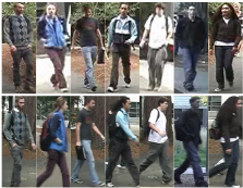
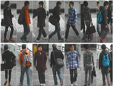
We test our proposed CBI 1 for person re-identification on two public datasets: VIPeR [Gray and Tao, 2008] and CUHK01 [Li et al., 2014]. Some example images of the two datasets are shown in Fig. 2. To illustrate the performance and efficiency of CBI, 17 recent algorithms, including 13 person reidentification methods and 4 multi-modal hash function learning methods, are used for comparison.
Image representation: In this paper, to reflect the advantage of our CBI to learn binary codes for different descriptors, three representations, including ELF [Gray and Tao, 2008], SCNCD [Yang et al., 2014] and LOMO [Liao et al., 2015], are adopted as the basic descriptors. CBI is not sensitive to the parameters for the two datasets and we set λ1 = 2 and C = 200 for all the experiments. However, λ2 will be set to 0▷05, 10 and 5 for ELF, SCNCD and LOMO, respectively.
Evaluation protocol: We randomly partition a dataset into two parts without overlap on person identities, according to a certain percentage. The expectation is reported by conducting 10 trials of evaluation. The parameters of other hashing algorithms are carefully tuned so that the best results are obtained. The results of other person re-identification methods either come from original papers or by running their offered codes, with exactly the same experimental setting. Same as most person re-identification publications, the standard Cumulated Matching Characteristics (CMC) [Wang et al., 2007] curves and the corresponding Area Under Curve (AUC) are used to illustrate the performance of different methods.
5.1 The efficiency of CBI
The Hamming distance comparison of the learned binary codes for two different persons in two views from the test set on the VIPeR dataset is shown in Fig. 3. According to the proposed CBI, binary codes with length 704 for each image are learned and resampled into an image with 22 ⇥ 32
1 The codes are released on a website:
https://sites.google.com/site/crossmodalhashing/re-identification
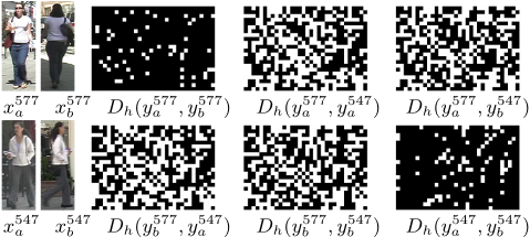
pixels so that it is easy to illustrate the difference of learned codes. From this figure, we can see that the Hamming distance between two images of a same person in two views is much lower than that between the images of different persons no matter they are captured in the same view or not.
CBI is efficient for similarity search in the testing stage, since the bit XOR operation is applied when calculating the Hamming distance. To illustrate the efficiency of CBI, we compare the time of similarity computation for various methods on the VIPeR dataset. To simulate a real situation, the time includes the feature projection for the probe image but the embedded features of gallery images are obtained in advance. All algorithms are run on a Matlab 7 platform installed on Windows 7 with Intel Core 3▷4GHz CPU and 8G memory. The codes of compared methods are provided by their original authors and comparison results are shown in Table 1. We can see that the proposed CBI is at least 2200 times faster than other methods. It is worth to point out that the local patches based methods, including eSDC [Zhao et al., 2013b], MLF [Zhao et al., 2014] and SalMatch [Zhao et al., 2013a], achieve advantageous performance (Rank 1: eSDC-26▷74%). However, the methods exploiting the local patches introduces a huge computational burden and they are 107 times slower than CBI. In general, in a real-world application, the number of samples in the gallery set n is very huge and the original dimension nd is much larger than the number of learned bits K. In theory, the efficiency of CBI is at least n(nd + 1)◁K times faster than other metric learning based methods.
5.2 Comparison with the state-of-the-art methods
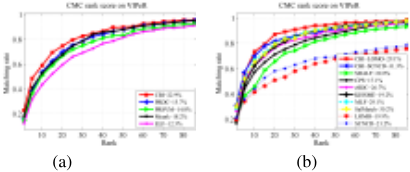
For evaluating on the VIPeR, we compare CBI with recent published algorithms, including: ELF [Gray and Tao, 2008], PRDC [Zheng et al., 2012], PRSVM [Prosser et al., 2010], SDALF [Farenzena et al., 2010], CPS [Cheng et al., 2011], Mrank [Loy et al., 2013], eSDC [Zhao et al., 2013b], SalMatch [Zhao et al., 2013a], MLF [Zhao et al., 2014], KISSME [Kostinger et al., 2012], SCNCD [Yang et al., 2014] and LOMO [Liao et al., 2015]. The comparison results are shown in Fig. 4 (a) and (b). Among them, PRDC, Mrank and PRSVM used the ELF feature. We can see that the proposed CBI achieves much better results than the three methods almost in all ranking. Following [Liao et al., 2015], a Cosine similarity measure is applied to SCNCD and LOMO. To compare with the three types of original features, we can see that the performance is boosted by CBI for at least 30%. Moreover, using the SCNCD feature, CBI is the best method at rank 1 and is better at low ranks ( 30) than other state-ofthe-art methods. Finally, by using LOMO feature, CBI has a 29▷1% accuracy at rank 1 and outperforms other methods almost at all ranks.
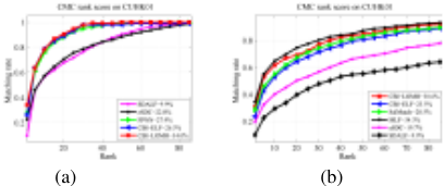
For comparing on the CUHK01, we follow two partitions as in [Li et al., 2014; Zhao et al., 2014] and the results are shown in Fig. 5. For the first partition with 100 test persons, three methods including FPNN [Li et al., 2014], eSDC [Zhao et al., 2013b] and SDALF [Farenzena et al., 2010] are compared with. We can see that CBI can achieve much better results than eSDC and SDALF at all ranks, no matter what features are used. To compare with the deep architecture based method FPNN, using the LOMO feature, CBI can achieve better results at all ranks while, using the SCNCD feature, is only slightly inferior FPNN at rank 1 (1.6 %) but better than FPNN at all other ranks. For the second partition with 486 test persons, the task is relatively more difficult and four state-ofthe-art methods including eSDC [Zhao et al., 2013b], SDALF [Farenzena et al., 2010], SalMatch [Zhao et al., 2013a] and MLF [Zhao et al., 2014] are compared against. In this setting, MLF is the best method but, using the LOMO feature, CBI achieves very similar performance to MLF. In fact, MLF is a local patches based method thus the computational burden of feature calculating and matching is very high.
In total, CBI can achieve competitive performance with the state-of-the-art methods. We have to point out that recent works on improved deep learning [Ahmed et al., 2015] and fusion based methods (LOMO+XQDA [Liao et al., 2015], MLF+LADF [Zhao et al., 2014], mixture of similarities [Chen et al., 2015] and ensemble of distances [Paisitkriangkrai et al., 2015]) reported higher results. However, since this paper mainly focuses on the efficiency, the combination of different methods is not considered, because they are computationally very expensive. Naturally, the performance of binary coding, a.k.a. hashing, methods will be lower than their corresponding non-hashing based methods due to the quantization loss [Gong and Lazebnik, 2011]. In the following section, the comparison of CCA [Hotelling, 1936] and CVH [Kumar and Udupa, 2011], which is a hashing version of CCA, will also prove this point. Therefore, we can conclude that, as a binary coding method for person re-identification, the performance of CBI is acceptable.
5.3 Comparison with other hashing methods
We compare our CBI with CCA [Hotelling, 1936] and multimodal binary code learning methods, including PDH [Rastegari et al., 2013], CVH [Kumar and Udupa, 2011], CMSSH [Bronstein and Bronstein, 2010] and CMFH [Ding et al., 2014] on the VIPeR and CUHK01 datasets.
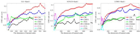
The comparison results at rank 1 are shown in Fig. 6. Firstly, due to the finite rank of variance matrix, the dimensions of the features learned by CCA and CVH are constrained, thus their best performance is poor. Secondly, at very low dimensions, most methods achieve similar results and the performance of CCA is better than others. Thirdly, the ranking scores of other three methods including CMFH, PDH and CMSSH do not progressively increase by the increase of the length of codes. This is because the later learned codes tend to add little discriminative information, due to ignoring the orthogonal constraint between different hash functions. Fourthly, our proposed method achieves much better results than other methods when the code length is over 400. Finally, Tables 2 and 3 show the best performance of each method with the optimal length of the learned codes. The overall AUC at ranks from 1 to 100 and the rank 1 accuracies have been reported. From the tables, we can see that CCA achieves much better results than the corresponding hashing version CVH. Moreover, we can observe that CBI outperforms all other binary code learning methods on the both datasets.
6 Conclusion
In this paper, a cross-view binary code learning method has been proposed for fast person re-identification. The main advantage of this method is that it hugely speeds up the procedure of the ranking or retrieval stage, when achieving equivalent performance to the state-of-the-art methods. Moreover, two more important points have also been observed. On the one hand, we firstly give an inside view of the intrinsic mechanism that the Hamming distance can be minimised by minimising the Euclidean distance when the learned linear hash functions satisfy the hinge loss constraint. In the future, it is meaningful to give a more compact boundary via the statistical perspective to enable a faster convergence of the algorithm. On the other hand, just dual modules have been used to learn the IDs of different persons. In fact, in a real world scenario, even in a building or a shopping mall, much more than two cameras are installed to monitor the human activities. Therefore, learning the IDs of persons from more than two views is useful. From this point of view, we can see that CBI is just a starting point in this area.
| Method | CBI | CMFH | PDH | CMSSH | CCA | CVH |
|---|---|---|---|---|---|---|
| ELF-AUC | 80.28 | 78.81 | 75.63 | 73.96 | 73.49 | 50.12 |
| SCNCD-AUC | 87.43 | 86.43 | 84.30 | 77.30 | 72.93 | 70.94 |
| LOMO-AUC | 89.92 | 88.80 | 84.06 | 85.04 | 79.96 | 58.77 |
| ELF-R1 | 0.221 | 0.165 | 0.117 | 0.114 | 0.083 | 0.063 |
| SCNCD-R1 | 0.313 | 0.222 | 0.225 | 0.165 | 0.218 | 0.158 |
| LOMO-R1 | 0.291 | 0.247 | 0.171 | 0.190 | 0.168 | 0.085 |
| Method | CBI | CMFH | PDH | CMSSH | CCA | CVH |
|---|---|---|---|---|---|---|
| ELF-AUC | 75.14 | 73.45 | 49.87 | 57.03 | 68.53 | 53.59 |
| LOMO-AUC | 80.63 | 79.78 | 49.81 | 57.58 | 73.63 | 52.45 |
| ELF-R1 | 0.235 | 0.150 | 0.056 | 0.102 | 0.156 | 0.065 |
| LOMO-R1 | 0.306 | 0.188 | 0.058 | 0.099 | 0.153 | 0.059 |
Appendix
Proof of Proposition 1
Proof: The Hamming distance between two binary codes ya and yb is defined by:
where 1(· ) is an indicator function. Thus, for any k, we consider two conditions: (1) If sign(wk a xa) = sign(wk b xb), it is obvious that
(2) If sign(wk a xa) 6= sign(wk b xb), we assume that sign(wk a xa) = 1 (Otherwise, same conclusion can be also obtained). There must be sign(wk b xb) = -1. Since the two linear projections are both hinge loss constraint satisfied functions, we have wk a xa ≥ 1-⇠ k a andwk b xb -1+⇠ k b . So, there is 2 - ⇠ k a - ⇠ k b ♣wk a xa - wk b xb♣. Provided that ⇠ k a + ⇠ k b 1, the following inequation is true:
In total, provided with 1(▷)2 = 1(▷), we obtain the following conclusion by satisfying 8k↪ ⇠ k a + ⇠ k b 1:
Proof of Proposition 3
Proof: The original objective function in Proposition 2 is:
If we fix all other variables except for wk a and ⇠ ki a , then the objective function and the constraints become:
If the orthogonal constraint of projections in intra-module has been added into the objective function using a balance parameter λ1, we obtain:
where Qka = Pj6=k wja (wja )T . If we set ⇥ka = λ1Qka + I and sbk ab = λ2Sabwk b , then we obtain:
Proof of Equation 10
Proof: For simplicity, we delete the subscripts of views and the index of projections k in this subsection. The optimal parameters wk a and ⇠ ki a can be obtained by solving the following objective function:
The objective function becomes a classical convex quadratic programming problem. To simplify the optimisation by transferring inequality constraints to equality constraints, a dual problem is designed. Thus, the Lagrange function can be defined as:
where e = (1↪ · · · ↪ 1)T , ⇠ = (⇠1↪ · · · ↪ ⇠n)T , ↵ = (⇠1↪ · · · ↪ ↵n)T , γ = (⇠1↪ · · · ↪ γn)T and Xy = (y1x1 ↪ · · · ↪ ynxn ). The gradient with respect to the parameters: @L @w = ⇥w-s-Xy ↵ and @L @⇠ = Ce-↵-γ. Then, the optimal values should satisfy the following constraints:
Substituting the above equations into the original Lagrange function, we obtain the dual problem:
@inproceedings{ijcai2016p342,
  title     = {Learning Cross-View Binary Identities for Fast Person Re-Identification},
  author    = {Zheng, Feng and Shao, Ling},
  booktitle = {Proceedings of the Twenty-Fifth International Joint Conference on
               Artificial Intelligence, {IJCAI-16}},
  publisher = {AAAI Press / International Joint Conferences on Artificial Intelligence},
  editor    = {Subbarao Kambhampati},
  pages     = {2399--2405},
  year      = {2016},
  month     = {7},
  url       = {https://ijcai.org/proceedings/2016/342},
}
TY - CPAPER TI - Learning Cross-View Binary Identities for Fast Person Re-Identification AU - Zheng, Feng AU - Shao, Ling T2 - Proceedings of the Twenty-Fifth International Joint Conference on Artificial Intelligence, IJCAI-16 PB - AAAI Press / International Joint Conferences on Artificial Intelligence PY - 2016 SP - 2399 EP - 2405 UR - https://ijcai.org/proceedings/2016/342 ER -Copied
Machine-readable versions of this paper, for tools and AI agents:





