
Probabilistic Rank-One Matrix Analysis with Concurrent Regularization
Proceedings of the Twenty-Fifth International Joint Conference on Artificial Intelligence. Pages 2428-2433.
Abstract
As a classical subspace learning method, Probabilistic PCA (PPCA) has been extended to several bilinear variants for dealing with matrix observations. However, they are all based on the Tucker model, leading to a restricted subspace representation and the problem of rotational ambiguity. To address these problems, this paper proposes a bilinear PPCA method named as Probabilistic Rank-One Matrix Analysis (PROMA). PROMA is based on the CP model, which leads to a more flexible subspace representation and does not suffer from rotational ambiguity. For better generalization, concurrent regularization is introduced to regularize the whole matrix subspace, rather than column and row factors separately. Experiments on both synthetic and real-world data demonstrate the superiority of PROMA in subspace estimation and classification as well as the effectiveness of concurrent regularization in regularizing bilinear PPCAs.
- [Ahn and Oh, 2003] J. Ahn and J. Oh. A constrained EM algo- rithm for principal component analysis. Neural Computation, 15(1):57-65, 2003.
- [Bishop, 1995] C. M. Bishop. Training with noise is equivalent to Tikhonov regularization. Neural computation, 7(1):108-116, 1995.
- [Carroll and Chang, 1970] J. D. Carroll and J. Chang. Analysis of individual differences in multidimensional scaling via an N-way generalization of Eckart-Young decomposition. Psychometrika, 35(3):283-319, 1970.
- [Chen et al., 2009] T. Chen, E. Martin, and G. Montague. Robust probabilistic PCA with missing data and contribution analysis for outlier detection. Computational Statistics & Data Analysis, 53(10):3706-3716, 2009.
- [Du et al., 2015] C. Du, S. Zhe, F. Zhuang, Y. Qi, Q. He, and Z. Shi. Bayesian maximum margin principal component anal- ysis. In Proc. of Twenty-Ninth AAAI Conf. on Artificial Intelli- gence, pages 2582-2588, 2015.
- [Duda et al., 2012] R. O. Duda, P. E. Hart, and D. G. Stork. Pattern Classification. John Wiley & Sons, 2012.
- [Gupta and Nagar, 1999] A. K. Gupta and D. K. Nagar. Matrix Variate Distributions, volume 104. CRC Press, 1999.
- [Harshman, 1970] R. A. Harshman. Foundations of the PARAFAC procedure: Models and conditions for an "explanatory" multi- modal factor analysis. UCLA Working Papers in Phonetics, 16:1- 84, 1970.
- [Jolliffe, 2002] I. T. Jolliffe. Principal Component Analysis. Springer Series in Statistics, second edition, 2002.
- [Khanna et al., 2015] R. Khanna, J. Ghosh, R. Poldrack, and O. Koyejo. Sparse submodular probabilistic PCA. In Proc. of the Eighteenth Int. Conf. on Artificial Intelligence and Statistics, pages 453-461, 2015.
- [Lu et al., 2008] H. Lu, K. N. Plataniotis, and A. N. Venetsanopou- los. MPCA: Multilinear principal component analysis of tensor objects. IEEE Trans. on Neural Networks, 19(1):18-39, 2008.
- [Lu et al., 2009] H. Lu, K. N. Plataniotis, and A. N. Venetsanopou- los. Uncorrelated multilinear principal component analysis for unsupervised multilinear subspace learning. IEEE Trans. on Neu- ral Networks, 20(11):1820-1836, 2009.
- [Lu et al., 2013] H. Lu, K. N. Plataniotis, and A. N. Venetsanopou- los. Multilinear Subspace Learning: Dimensionality Reduction of Multidimensional Data. CRC Press, 2013.
- [Meng and Rubin, 1993] X. Meng and D. B. Rubin. Maximum likelihood estimation via the ECM algorithm: A general frame- work. Biometrika, 80(2):267-278, 1993.
- [Phillips et al., 2000] P. J. Phillips, H. Moon, S. A. Rizvi, and P. Rauss. The FERET evaluation method for face recognition algorithms. IEEE Trans. on Pattern Analysis and Machine Intel- ligence, 22(10):1090-1104, 2000.
- [Shan et al., 2011] H. Shan, A. Banerjee, and R. Natarajan. Proba- bilistic tensor factorization for tensor completion. Technical Re- port TR 11-026, Department of Computer Science and Engineer- ing, University of Minnesota, 2011.
- [Shashua and Levin, 2001] A. Shashua and A. Levin. Linear im- age coding for regression and classification using the tensor-rank principle. In Proc. of IEEE Int. Conf. on Computer Vision and Pattern Recognition, volume I, pages 42-49, 2001.
- [Sim et al., 2003] T. Sim, S. Baker, and M. Bsat. The CMU pose, illumination, and expression database. IEEE Trans. on Pattern Analysis and Machine Intelligence, 25(12):1615-1618, 2003.
- [Tipping and Bishop, 1999] M. E. Tipping and C. M. Bishop. Prob- abilistic principal component analysis. Journal of the Royal Sta- tistical Society: Series B (Statistical Methodology), 61(3):611- 622, 1999.
- [Tucker, 1966] L. R. Tucker. Some mathematical notes on three- mode factor analysis. Psychometrika, 31(3):279-311, 1966.
- [Xie et al., 2008] X. Xie, S. Yan, J. T. Kwok, and T. S. Huang. Matrix-variate factor analysis and its applications. IEEE Trans. on Neural Networks, 19(10):1821-1826, 2008.
- [Xiong et al., 2010] L. Xiong, X. Chen, T. Huang, J. G. Schnei- der, and J. G. Carbonell. Temporal collaborative filtering with Bayesian probabilistic tensor factorization. In Proc. of SIAM Int. Conf. on Data Mining, volume 10, pages 211-222. SIAM, 2010.
- [Xu et al., 2005] D. Xu, S. Yan, L. Zhang, H.-J. Zhang, Z. Liu, and H.-Y. Shum;. Concurrent subspaces analysis. In Proc. of IEEE Int. Conf. on Computer Vision and Pattern Recognition, volume II, pages 203-208, 2005.
- [Yang et al., 2004] J. Yang, D. Zhang, A. F. Frangi, and J. Yang. Two-dimensional PCA: a new approach to appearance-based face representation and recognition. IEEE Trans. on Pattern Analysis and Machine Intelligence, 26(1):131-137, 2004.
- [Ye et al., 2004] J. Ye, R. Janardan, and Q. Li. GPCA: An effi- cient dimension reduction scheme for image compression and retrieval. In Proc. of ACM SIGKDD Int. Conf. on Knowledge Discovery and Data Mining, pages 354-363, 2004.
- [Ye, 2005] J. Ye. Generalized low rank approximations of matrices. Machine Learning, 61(1-3):167-191, 2005.
- [Yu et al., 2011] S. Yu, J. Bi, and J. Ye. Matrix-variate and higher- order probabilistic projections. Data Mining and Knowledge Dis- covery, 22(3):372-392, 2011.
- [Zhao et al., 2012] J. Zhao, P. L. H. Yu, and J. T. Kwok. Bilinear probabilistic principal component analysis. IEEE Trans. on Neu- ral Networks and Learning Systems, 23(3):492-503, 2012.
- [Zhao et al., 2015] Q. Zhao, L. Zhang, and A. Cichocki. Bayesian CP factorization of incomplete tensors with automatic rank de- termination. IEEE Trans. on Pattern Analysis and Machine Intel- ligence, 37(9):1751-1763, 2015.
References were extracted automatically from the PDF and may contain errors.
Full text extracted automatically from the PDF; figures, tables and equations may differ. The PDF is the version of record.
1 Introduction
Principal Component Analysis (PCA) [Jolliffe, 2002] is a classical subspace learning technique. It is widely used for various applications such as data compression, computer vision, and pattern recognition. Probabilistic PCA (PPCA) [Tipping and Bishop, 1999] is an important extension of PCA. It reformulates PCA as a generative model, which brings two main advantages: 1) It can capture data uncertainty and handle missing values; 2) By introducing proper prior distributions, it enables automatic model selection or incorporation of desired properties such as robustness [Chen et al., 2009], sparsity [Khanna et al., 2015], and large-margin separability [Du et al., 2015]. Although PCA and PPCA have wide applications, they are designed for vector inputs, and require vectorization (reshaping) to deal with multidimensional data. This may lead to some loss of data information due to the broken spatial structures.
To address the above problem, various multilinear extensions of PCA have been proposed, where the input data are represented by tensors (multidimensional arrays). Roughly speaking, multilinear PCA methods can be grouped into two branches [Lu et al., 2013]. One is based on the Tucker model [Tucker, 1966] that learns low-dimensional tensors from high-dimensional tensors [Yang et al., 2004; Ye, 2005; Ye et al., 2004; Xu et al., 2005; Lu et al., 2008]. The other branch is based on the CANDECOMP/PARAFAC (CP) model [Carroll and Chang, 1970; Harshman, 1970] that learns low-dimensional vectors from high-dimensional tensors, in a successive way [Shashua and Levin, 2001; Lu et al., 2009].
Several attempts have also been made to take advantages of both probabilistic models and tensor representations. This paper focuses on bilinear extensions of PPCA, which aims to learn a subspace from matrix (second-order tensor) inputs. Matrix-Variate Factor Analysis (MVFA) [Xie et al., 2008] may be the first bilinear PPCA method. It relates each (matrix) observation to a low-dimensional latent matrix via introducing column and row factor matrices. With the same spirit as MVFA, Probabilistic Second-Order PCA (PSOPCA) [Yu et al., 2011] provides a probabilistic interpretation of bilinear PCAs by assuming that both matrix observations and latent matrices are from matrix-variate normal distributions [Gupta and Nagar, 1999]. By adding two extra noise terms to the PSOPCA model, Bilinear Probabilistic PCA (BPPCA) [Zhao et al., 2012] can analytically marginalize out latent matrices and provide closed-form updates for both maximum likelihood estimation (MLE) and maximum a posteriori (MAP) estimation.
All the existing bilinear PPCA methods are Tucker-based. They have a restricted subspace representation that reuses each column/row factor for constructing multiple bases of the matrix subspace. This enables them to model the matrix subspace with only a small number of parameters, but also limits the flexibility in capturing data characteristics. In addition, like PPCA, Tucker-based PPCAs suffer from rotational ambiguity [Tipping and Bishop, 1999; Ahn and Oh, 2003], which means that they can only estimate the span rather than the exact axes of the underlying subspace. This is undesirable for applications such as data interpretation and visualization [Jolliffe, 2002].
To address the above problems of Tucker-based bilinear PPCAs, this paper proposes a bilinear PPCA method based on the CP model, named as Probabilistic Rank-One Matrix Analysis (PROMA). PROMA models each observation as a linear combination of rank-one matrices, and does not suffer from rotational ambiguity. Moreover, it takes the Tuckerbased PPCA model as a special case, providing more flexibility in capturing data characteristics. To obtain robust solutions against overfitting, we need regularization in PROMA. Instead of separately regularizing column and row factors, we propose concurrent regularization to penalize the whole matrix subspace and relax the scale restriction of separate regularization, which could lead to better generalization for CPbased PPCAs.
2 Preliminaries
This section describes the notations and definitions needed in the proposed method, and provides a brief review on PPCA and its bilinear extensions.
Notations: Vectors and matrices are denoted by bold lowercase (x) and uppercase (X) letters, respectively. Superscript > denotes the transposition. Symbols ⌦ and ~ denote the Kronecker and Hadamard (entrywise) product, respectively. ⊙ is the Khatri-Rao (column-wise Kronecker) product of two matrices C = (c1↪ ▷ ▷ ▷ ↪ cP ) 2 Rdc⇥P and R = (r1↪ ▷ ▷ ▷ ↪ rP ) 2 Rdr⇥P , which leads to a dcdr ⇥ P matrix denoted as C ⊙ R whose pth column is cp ⌦ rp (p = 1↪ ▷ ▷ ▷ ↪ P). h·i denotes the expectation w.r.t. a certain distribution. tr(·) is the matrix trace, vec(·) is the vectorization operator that stacks the columns of a matrix into a single column vector, and diag(·) is the operator that creates a diagonal matrix from a vector or a vector formed by the diagonal elements of a matrix. Ndc↪dr (⌅↪⌃c↪⌃r) denotes a matrix-variate normal distribution with the mean matrix ⌅, covariance matrices ⌃c 2 Rdc⇥dc and ⌃r 2 Rdr⇥dr , which is related to the multivariate normal distribution in the following way: X⇠Ndc↪dr (⌅↪⌃c↪⌃r) if and only if vec(X) ⇠ N (vec(⌅)↪ ⌃r ⌦ ⌃c) [Gupta and Nagar, 1999].
PPCA model: PPCA relates a d-dimensional observation vector x to a q-dimensional latent vector z as follows:
where W 2 Rd⇥q is the factor loading matrix, ✏ ⇠N(0↪ σ2 I) represents random noise with variance σ2 , z ⇠ N(0↪ I) is independent of ✏ , and θ is the mean vector. In essence, the goal of PPCA is to learn a q-dimensional subspace spanned by the columns of W from d-dimensional observations. When the observation X 2 Rdc⇥dr is in the matrix form, we need to vectorize X first, and then perform PPCA on vec(X) 2 Rdc·dr .
Tucker-based bilinear PPCA model: Bilinear PPCA methods such as PSOPCA and BPPCA take matrices as inputs without vectorization. They are all based on the Tucker model, which relates each matrix observation with a latent matrix. Specifically, they aim to find a qc · qr-dimensional subspace by modeling a matrix observation X as follows:
where Z 2 Rqc⇥qr is a latent matrix with Z ⇠ Nqc↪qr (0↪ I↪ I) serving as the low-dimensional representation of X, ⌅ is the mean matrix, and E 2 Rdc⇥dr is a noise matrix and independent of Z. Each element of E is an independent identically distributed (i.i.d.) normal random variable with Eij ⇠ N(0↪ σ2 ), which is also equivalent to E ⇠ Ndc↪dr (0↪ σI↪ σI) with σ > 0. Uc = (uc1 ↪ ▷ ▷ ▷ ↪ ucqc ) and Ur = (ur1 ↪ ▷ ▷ ▷ ↪ urqr ) are the column and row factor matrices, respectively.
Compared with the PPCA model (1), Tucker-based one (2) requires much fewer parameters (Uc and Ur rather thanW) to model the same number of latent features, while, as will be seen in the next section, this subspace representation is relatively restricted and has limited flexibility in capturing data characteristics.
3 Probabilistic Rank-One Matrix Analysis with Concurrent Regularization
This section presents our Probabilistic Rank-One Matrix Analysis (PROMA) method in three stages: 1) We introduce a CP-based bilinear PPCA Model, which is more general than the Tucker-based one (2); 2) concurrent regularization is proposed to alleviate overfitting for CP-based PPCAs; 3) we develop the PROMA algorithm with a data-dependent strategy of determining the regularization parameter.
3.1 CP-Based Bilinear PPCAModel
We assume that an observed matrix X can be represented by a linear combination of P rank-one matrices, whose coefficients are the elements of a latent vector z 2 RP . This leads to a CP model as follows:
where zp is the pth element of z ⇠N(0↪ I), and E ⇠Ndc↪dr (0↪ σI↪ σI) with σ > 0. C = (c1↪ ▷ ▷ ▷ ↪ cP ) 2 Rdc⇥P and R = (r1↪ ▷ ▷ ▷ ↪ rP ) 2 Rdr⇥P are the column and row factor matrices, respectively.
Despite of modeling data in different ways, (1), (2), and (3) have the same goal of learning a subspace from vec(X) or X. In the following discussions, we study different PPCA models in a typical subspace learning setting, where the dimensionality of the matrix subspace or the number of latent features is given, i.e. q = qc · qr = P.
Connections with PPCA: We first explore the connections between PPCA and its bilinear extensions.
Proposition 1. Given q = qc · qr = P, the Tucker and CP models (2) and (3) are equivalent to the PPCA model (1) with W=Ur ⌦Uc and R⊙C, respectively.
Proof. By vectorizing both sides of (2) and (3), and using the fact that vec(UcZUr>) = (Ur ⌦ Uc )vec(Z), the Tucker model (2) can be rewritten as follows:
With vec(zpcprp>) = zprp ⌦cp, the CP model (3) becomes:
Since z = vec(Z) ⇠ N(0↪ I), θ = vec(⌅), and ✏ = vec(E) ⇠ N(0↪ σ2 I), (2) and (3) are equivalent to the PPCA model (1) with W = Ur ⌦Uc for the Tucker model, and W = (r1⌦c1↪ ▷ ▷ ▷ ↪ rP ⌦cP ) = R⊙C for the CP model.
Proposition 1 implies that both the Tucker- and CP-based PPCAs can be viewed as PPCA with a specific parameterization of the factor matrixW. This also means that inferring the Tucker and CP models is equivalent to estimating a subspace spanned by the columns of Ur ⌦Uc and R⊙C, respectively.
Connections with Tucker-based bilinear PPCAs: Next, we will show that in the same setting of subspace learning, the Tucker model (2) is a special case of the CP model (3).
Theorem 1. Given P = qc · qr, the Tucker model (2) is a special case of the CP model (3).
Proof. The Tucker model (2) can be rewritten as the following summation form of the CP model (3):
where z = vec(Z), ˆC = (uc1 ↪ ▷ ▷ ▷ ↪ uc1 ↪ ▷ ▷ ▷ ↪ ucqc ↪ ▷ ▷ ▷↪ ucqc ), and ˆR = (Ur ↪ ▷ ▷ ▷ ↪Ur ). Therefore, the Tucker model is just a CP model with qr and qc repeated uci (i = 1↪ ▷ ▷ ▷ ↪ qc) and urj (j = 1↪ ▷ ▷ ▷ ↪ qr) in C and R, respectively.
From Proposition 1 and Theorem 1, the Tucker model (2) represents the matrix subspace as Ur ⌦ Uc = ˆR ⊙ ˆC = (ur1 ⌦ uc1 ↪ ur2 ⌦ uc1 ↪ ▷ ▷ ▷ ↪ urqr ⌦ uc1 ↪ ur1 ⌦ uc2 ↪ ▷ ▷ ▷ ↪ urqr ⌦ ucqc ). It reuses each column of Uc and Ur to construct multiple bases of the matrix subspace. This makes each subspace basis constructed by uci and urj (i = 1↪ ▷ ▷ ▷ ↪ qc; j = 1↪ ▷ ▷ ▷ ↪ qr) share some common information with (qc - 1) + (qr - 1) other bases, leading to restricted flexibility in capturing data characteristics. In contrast, the CP model (3) does not have this restriction and allows each subspace basis rp ⌦ cp to be constructed by distinct pair of factors. Thus, it generalizes the Tucker model (2), and has more potential of capturing useful data characteristics.
Log-likelihood function: Armed with the CP model (3), the conditional distribution of X given z is as follows:
which is also equivalent to vec(X)♣z ⇠ N((R ⊙ C)z + θ↪ σ2 I). Without loss of generality, we assume that data are centered and thus ⌅ = 0. Given a set of observations ¶Xn♦Nn=1 , we can take the expectation of the complete-data log-likelihood L = PNn=1 lnp(Xn↪ zn) w.r.t. the conditional distribution p(z♣X). Defining the parameter set ✓ = ¶C↪ R↪ σ2 ♦, we have
With the above log-likelihood function, we can estimate the model parameters by maximizing (5) w.r.t. ✓.
Rotational ambiguity avoided: Apart form its flexibility, another advantage of the CP model over the Tucker one is that it does not suffer from rotational ambiguity. This means that maximizing the likelihood function (5) leads to unique C and R up to rotation transformations, which results in the optimal axes of the matrix subspace in the sense of maximum likelihood. This property could be very useful in data interpretation and visualization. In contrast, Tucker-based bilinear PPCAs have rotational ambiguity and can only obtain arbitrary bases spanning the subspace, since their solutions with and without rotation transformations are equally good in terms of the likelihood function [Zhao et al., 2012].
3.2 Regularization for CP-based PPCAs
In order to obtain robust solutions against overfitting, it is common to regularize the log-likelihood function (5) by adding certain regularization terms for C and R or introducing priori distributions over C and R separately.
Separate regularization: For clarity, we only discuss L2 regularization for penalizing smoothness, while similar conclusions can also be drawn for more general regularizations. It would be natural to regularize the log-likelihood function (5) as follows:
where γc and γr are regularization parameters. This is equivalent to introducing Gaussian priori distributions p(C♣γc) = QPp=1 N (cp♣0↪ γ-1 c I) and p(R♣γr) = QPp=1 N(rp♣0↪ γ-1 r I) over the factor matrices C and R, respectively.
Scale restriction: However, this conventional approach is not good enough for CP-based PPCAs, because C and R are penalized separately. Recall from Proposition 1 that the CP model learns a subspace spanned by the columns of W = R ⊙ C. Although W is constructed by C and R, we eventually favor a smoothed W, whereas imposing smoothness on C and R separately may not lead to a smoothed W. Moreover, due to the regularization terms ♣♣cp♣♣2 and ♣♣rp♣♣2 , (6) restricts the scales of cp and rp to specific values. However, this restriction seems unnecessary, because (5) is invariant to scale transformations cp 7! scp, rp 7! s-1 rp (s 6= 0) and does not prefer certain scales of cp and rp. Consequently, regularizing C and R separately may exclude some good solutions in terms of (5). Can we relax such restriction in regularizing CP-based PPCAs?
Concurrent regularization: Bishop [1995] proved that adding random noise to the training examples is equivalent to Tikhonov regularization. This inspires us to regularize CP-based PPCAs via introducing additional noise. Instead of generating a noisy training set as [Bishop, 1995], we introduce additional noise by adjusting the noise variance σ2 . Specifically, we replace σ2 in (5) with a regularization parameter γ. Varying the noise level can balance the influences between observations with high likelihood values and those with low ones, which in turn improves robustness against overfitting. In the context of fitting the CP model, the additional noise regularizes C and R at the same time. Therefore, we name this strategy concurrent regularization.
Unlike separate regularization, concurrent regularization does not restrict the scales of cp and rp. Thus it is more flexible in regularizing CP-based PPCAs, and has potential to find better solutions. Concurrent regularization can also be viewed as a bias-variance trade-off of the CP model, where we improve the generalization performance by increasing the bias of fitting training data (reflected by γ).
3.3 PROMAAlgorithm
This section develops the PROMA algorithm that combines the CP model with concurrent regularization. Note that it is difficult to maximize (5) w.r.t. both C and R, because they are coupled with each other. To address this problem, we sequentially and conditionally maximizes (5) w.r.t. C and R following the expectation-conditional maximization (ECM) approach [Meng and Rubin, 1993]. Specifically, PROMA consists of two steps: the Regularized Expectation (RE-step) and the Conditional Maximization (CM-step).
RE-step: We first evaluate the expectation hzni and hznz>n i w.r.t. the conditional distribution p(zn♣Xn) (or p(zn♣vec(Xn)) equivalently) for each Xn. Using Bayes' rule with θ = vec(⌅) = 0, we have
where W = R ⊙ C, and M = W>W + γI = C>C ~ R>R+γI is a P ⇥P matrix. Based on (7), we can compute hzni and hznz>n i with the current fixed values of the model parameters as follows:
where γ is the parameter introduced by concurrent regularization, leading to a Regularized E-step. An appropriate γ regularizes the whole subspace via W>W+ γI, and solves ill-conditioned problems of M-1 . This in turn leads to more robust hzni and hznz>n i against overfitting.
CM-step: We then maximize the log-likelihood function (5) w.r.t. C (or R) with the other fixed. By fixing R, we maximize (5) w.r.t. C and obtain:
With a similar derivation as ˜C, we have
By alternatively iterating between the RE-step and CM-step, we can find the MLE solutions ˆC and ˆR. Then the latent representation z of an observation X can be computed via hz♣Xi = M-1 diag( ˆC>X ˆR). Algorithm 1 is the pseudocode of PROMA. It always increases the log-likelihood function (5) and is guaranteed to converge [Meng and Rubin, 1993].
Connections with Bayesian CP decomposition: Bayesian CP decomposition methods [Xiong et al., 2010; Shan et al., 2011; Zhao et al., 2015] share the same CP model as PROMA, while they focus on transductive inferences of estimating the marginal distribution p(X). In contrast,
Algorithm 1 Probabilistic Rank-One Matrix Analysis
- 1: Input: Data set ¶Xn 2 Rdc⇥dr ♦Nn=1, the number of extracted features P, the maximum number of iterations K, and the concurrent regularization parameter γ.
- 2: Initialize C and R randomly, and normalize each column of C and R to have unit norm.
- 3: repeat
- 4: Compute the conditional expectations hzni and hznz>n i via (8) and (9), respectively.
- 5: Update C and R via (10) and (11), respectively.
- 6: until convergence or after K iterations.
- 7: Output: The factor matrices C and R.
PROMA aims to project high-dimensional data into a lowdimensional subspace, which requires inductive inferences of estimating the conditional distribution p(z♣X). Therefore, it is non-trivial to apply Bayesian CP decomposition for subspace learning because p(z♣X) is generally intractable based on Bayesian inference. Moreover, PROMA is equipped with concurrent regularization, while Bayesian CP decomposition methods separately regularize individual factor matrices with priori distributions.
Parameter initialization: We use a random scheme to initialize PROMA, where each column of C and R is randomly drawn from N(0↪ I). Such initialization puts a random weight on each column of W = R ⊙ C, which will make PROMA favor certain pairs of factors and bias the final results. Thus, the columns of C and R are normalized to have unit norm, so that the initialized factors are equally weighted.
PROMA NR algorithm: Notice that if σ2 is still estimated by maximizing the log-likelihood function (5) rather than being replaced by γ, No concurrent Regularization is imposed, and we name this algorithm PROMA NR . Specifically, maximizing (5) w.r.t. σ2 leads to
Therefore, PROMA NR is just PROMA with γ = σ2 updated according to (12) in each iteration, where σ2 can be initialized randomly.
Automatic determination of γ: PROMA involves the regularization parameter γ. Cross-validation can be used for parameter determination, while it could be time consuming. Here, we propose a data-dependent strategy to find a reasonably good γ for PROMA. Specifically, we determine γ by performing PROMA NR with P = 1. This provides a onedimensional search of total data variance captured by the CP model, where data are projected into a one-dimensional subspace. We find this strategy works well empirically, and is also very efficient because PROMA NR with P = 1 is very fast and converges within a few iterations.
4 Experiments
This section evaluates PROMA against competing methods on both synthetic and real-world data sets.
| Method | PSOPCA | BPPCA | PROMA NR | PROMA |
|---|---|---|---|---|
| Arc length | 3.67 | 3.98 | 9.70e-8 | 5.56e-5 |
| distance |
distance ◦0.04 ◦0.09 ◦1.46e-8 ◦1.43e-5
4.1 Subspace Estimation on Synthetic Data
We generate synthetic 2-D data sets from the CP model (3) as follows: two factor matrices C⇤ and R⇤ are generated by drawing each row of C⇤ and R⇤ from a Gaussian distribution N(0↪ IP ⇤). Then N = 1000 latent vectors ¶z⇤n 2 RP ⇤ ♦Nn=1 are drawn from N(0↪ IP ⇤), and the observed matrices with a size of 30 ⇥ 30 are constructed by Xn = C⇤ diag(z⇤n )R⇤> without noise. According to Proposition 1, the synthetic data lie in the subspace spanned by the columns of W⇤ = R⇤ ⊙ C⇤ . Our aim is to evaluate the subspace estimation accuracy by comparing the arc length distance between the estimated subspace W and the true one W⇤ . This distance measures the angle between subspaces, and is defined as ♣♣β♣♣2, where β = (β1↪ ▷ ▷ ▷ ↪ βP ⇤), and ¶cos(βp)♦P ⇤ p=1 are the singular values ofW>W⇤ [Zhao et al., 2012].
We compare PROMA NR , and PROMA (γ = 0▷05) against Tucker-based PPCAs including PSOPCA and BPPCA on 10 randomly generated synthetic data sets with P ⇤ = 9. PROMA NR and PROMA with P = 9, and PSOPCA and BPPCA with qc = 3↪ qr = 3 are performed to estimate the true P ⇤ -dimensional subspace. Table 1 shows the average subspace estimation accuracy of different algorithms. It is clear that PROMA NR almost perfectly estimates the true subspace, whereas PSOPCA and BPPCA fail to estimate the subspace accurately.
PROMA also gets good results in Table 1 but is worse than PROMA NR , because concurrent regularization introduces additional noise, and reduces the model fit for the ideal data. However, real-world data are usually noisy and not perfectly generated from the CP model. In this case, concurrent regularization, as will be seen, is effective in alleviating overfitting for not only PROMA but also other bilinear PPCAs.
4.2 Classification on Real-World Data
Two face data sets are tested. The first one is a subset of the FERET database [Phillips et al., 2000] including all subjects with at least eight images and at most 15 degrees of pose variation, resulting in 721 face images from 70 subjects.
The second one is a subset from the PIE database [Sim et al., 2003], with seven poses (C05, C07, C09, C27, C29, C37, C11) of at most 45 degrees of pose variation and under 21 illumination conditions (02 to 22). This subset contains 9,987 face images from 68 subjects. Each face image is normalized to 32 ⇥ 32 graylevel pixels.
Algorithms and their settings: We compare PROMA NR and PROMA against linear baselines: PCA, PPCA; Tuckerbased PCA: MPCA [Lu et al., 2008]; CP-based PCAs: TROD [Shashua and Levin, 2001], UMPCA [Lu et al., 2009], and Tucker-based PPCAs: PSOPCA, BPPCA. For completeness, Bayesian CP factorization (BCPF) [Zhao et al., 2015]
is also compared, where the conditional expectation of (8) is used to perform dimensionality reduction. We also test PSOPCA and BPPCA with Concurrent Regularization as well as PROMA NR with Separate Regularization, denoted by PSOPCA CR , BPPCA CR , and PROMA SR , respectively. We show their best results, where the regularization parameters are selected from ¶10-4 ↪ 10-3 ↪ ▷ ▷ ▷ ↪ 104 ♦.
PCA and MPCA are performed to preserve 97% energy, while changing the value of preserved energy of PCA and MPCA from 95 ⇠ 99% leads to similar results. For PPCA, UMPCA, PSOPCA, and BPPCA, we test up to 1023, 32, 961, and 961 features, respectively, which are the maximum numbers that can be extracted. We test up to P = 600 features for TROD, BCPF, PROMA NR , PROMA SR and PROMA, since their numbers of extracted feature are not bounded by the input dimensions. For MPCA, TROD, and UMPCA, we use their default settings with up to 1↪ 10, and 10 iterations, respectively. BPPCA has both MLE and MAP implementations. We choose the MLE-based one used in face recognition [Zhao et al., 2012] by iterating until convergence. We iterate PROMA NR , PROMA SR , and PROMA until convergence or 500 iterations. The regularization parameter γ of PROMA is automatically determined by PROMA NR with P = 1.
Experiment setup: We randomly split the FERET and PIE data sets into training and test sets so that each subject has L images for training, and the rest are used for test. We report the results over ten such random splits. After feature extraction via each method, all the features are sorted according to the Fisher score [Duda et al., 2012] in descending order, and then the nearest neighbor classifier is used to obtain the recognition rates. For each method and L, we report the best recognition rates obtained using different numbers of the extracted features (up to the maximums) in Tables 2 and 3. We highlight the best and comparable results in bold font based on t-test with a p-value of 0▷01, and underline the second best ones.
Recognition results: Tables 2 and 3 show the recognition results on the FERET and PIE data sets, respectively. PROMA consistently achieves the best results with statistical significance on the whole, while PROMA SR seems the second best method. PROMA outperforms BPPCA (BPPCA CR ), the best Tucker-based PPCA, by 5.44% (3.59%) and 5.13% (4.64%) on average for the FERET and PIE data sets, respectively. This could be attributed to the CP model in charactering the underlying subspace with more flexibility as well as the concurrent regularization in alleviating overfitting. On the other hand, although it already imposes regularization, BCPF does not work well in all the cases, which indicates that applying tensor decomposition methods for subspace learning is not a trivial task.
Effectiveness of concurrent regularization: Concurrent regularization significantly improves PROMA NR by 17.65% and 11.68% on average for the FERET and PIE data sets, respectively. It also improves Tucker-based PPCAs, PSOPCA and BPPCA, in most cases. By optimizing regularized log-likelihood function (6), PROMA SR always outperforms PROMA NR , while it is still inferior to PROMA. This could be attributed to concurrent regularization in penalizing the whole
Table 2: Recognition rates (Mean◦Std.%) on the FERET data set (Best; Second best).
67.49◦2.59
| L | 2 | 3 | 4 | 5 | 6 | 7 |
|---|---|---|---|---|---|---|
| PCA | 46.49◦3.43 | 54.09◦4.88 | 59.71◦2.62 | 67.39◦3.36 | 71.40◦2.40 | 72.16◦3.35 |
| PPCA | 51.14◦1.99 | 63.78◦3.02 | 69.18◦3.44 | 73.69◦0.66 | 77.94◦2.73 | 77.88◦2.79 |
| MPCA | 57.56◦3.69 | 67.73◦1.87 | 72.04◦2.10 | 76.60◦2.25 | 79.73◦2.55 | 81.08◦2.40 |
| UMPCA | 47.72◦5.62 | 57.83◦4.18 | 64.29◦3.53 | 69.87◦4.72 | 73.72◦5.08 | 75.24◦2.12 |
| TROD | 61.62◦2.92 | 69.49◦3.29 | 74.65◦3.00 | 79.11◦1.50 | 81.89◦1.98 | 83.55◦2.26 |
| BCPF | 52.67◦2.12 | 62.72◦3.24 | 68.62◦2.52 | 74.04◦1.51 | 77.24◦2.42 | 79.83◦2.88 |
| PSOPCA | 51.51◦2.10 | 60.47◦2.60 | 65.96◦3.04 | 70.89◦2.41 | 74.49◦2.45 | 75.89◦3.17 |
| PSOPCA CR | 59.02◦2.35 | 68.18◦2.16 | 72.83◦2.66 | 77.47◦1.83 | 80.20◦1.84 | 81.26◦2.39 |
| BPPCA | 62.10◦3.39 | 71.06◦3.45 | 76.67◦3.34 | 81.97◦1.44 | 84.52◦2.36 | 85.19◦2.13 |
| BPPCA CR | 64.30◦2.82 | 73.29◦2.25 | 77.69◦2.31 | 82.35◦1.12 | 84.95◦2.19 | 87.23◦2.09 |
| PROMA NR | 49.21◦2.37 | 56.99◦2.28 | 62.54◦3.59 | 68.84◦1.23 | 72.52◦3.51 | 75.32◦2.41 |
| PROMA SR | 64.25◦3.25 | 73.01◦2.88 | 79.09◦2.43 | 83.32◦2.64 | 86.98◦2.85 | 86.54◦2.49 |
| PROMA |
77.16◦2.13
82.56◦3.52
85.55◦1.82
88.84◦2.07
89.74◦2.15
Table 3: Recognition rates (Mean◦Std.%) on the PIE data set (Best; Second best).
42.42◦1.74 53.85◦1.71 59.91◦1.73 65.77◦1.62 69.13◦1.27 75.28◦1.18 79.13◦0.91 89.36◦0.67
| L | 2 | 3 | 4 | 5 | 6 | 8 | 10 | 20 |
|---|---|---|---|---|---|---|---|---|
| PCA | 26.41◦3.35 | 37.25◦1.50 | 43.04◦2.51 | 49.50◦2.14 | 52.08◦2.58 | 60.68◦1.74 | 66.26◦0.87 | 82.40◦0.64 |
| PPCA | 24.41◦2.14 | 38.00◦0.94 | 45.48◦1.82 | 51.24◦0.93 | 55.54◦0.99 | 64.25◦1.25 | 69.82◦0.48 | 86.66◦3.06 |
| MPCA | 35.27◦2.97 | 46.25◦2.56 | 51.74◦1.79 | 56.61◦1.63 | 59.60◦0.58 | 66.75◦0.66 | 71.48◦0.66 | 84.35◦1.48 |
| UMPCA | 29.08◦3.06 | 38.11◦2.11 | 42.52◦3.42 | 48.34◦3.03 | 51.04◦3.05 | 58.12◦3.31 | 61.61◦3.24 | 76.38◦2.39 |
| TROD | 34.52◦1.84 | 42.92◦2.75 | 47.90◦2.52 | 52.92◦1.87 | 56.33◦1.52 | 63.30◦0.93 | 67.70◦1.21 | 81.07◦1.54 |
| BCPF | 31.56◦1.13 | 42.63◦1.81 | 50.00◦1.92 | 57.13◦1.79 | 61.39◦0.75 | 69.55◦0.70 | 74.69◦0.60 | 81.27◦1.10 |
| PSOPCA | 31.09◦3.10 | 39.21◦3.07 | 45.79◦2.98 | 52.38◦2.64 | 56.60◦2.79 | 63.99◦2.41 | 68.76◦2.19 | 84.37◦1.50 |
| PSOPCA CR | 35.15◦1.23 | 44.92◦1.23 | 50.61◦2.05 | 56.02◦1.16 | 60.32◦1.02 | 67.77◦0.81 | 71.71◦1.16 | 85.72◦0.65 |
| BPPCA | 36.07◦1.88 | 47.41◦1.93 | 53.23◦2.39 | 59.25◦2.27 | 63.84◦1.81 | 71.14◦1.13 | 74.83◦2.00 | 88.06◦0.95 |
| BPPCA CR | 37.39◦2.65 | 47.67◦1.91 | 54.03◦2.37 | 60.53◦1.99 | 63.91◦1.88 | 71.35◦2.59 | 75.09◦0.83 | 87.78◦0.94 |
| PROMA NR | 27.59◦1.12 | 36.14◦1.18 | 43.86◦1.62 | 51.32◦1.39 | 56.30◦1.02 | 66.07◦0.96 | 72.11◦0.64 | 88.01◦1.04 |
| PROMA SR | 36.83◦1.81 | 47.82◦1.73 | 55.10◦2.03 | 61.59◦1.24 | 65.47◦1.25 | 72.49◦1.18 | 76.12◦0.82 | 89.08◦0.71 |
| PROMA |
matrix subspace and relaxing the scale restriction of separate regularization.
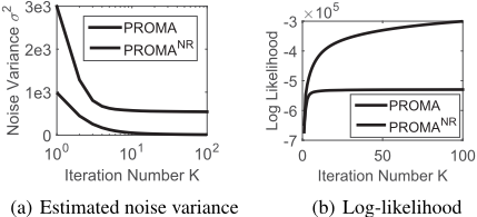
Goodness-of-fit: It is worth noting that although PROMA replaces the noise variance σ2 with the regularization parameter γ, we can still calculate σ2 for PROMA according to (12), whose value indicates how well the CP model fits the training data. Figure 1(a) shows the noise variance σ2 of PROMA NR and PROMA w.r.t. the iteration number K on the FERET data set with L = 2. PROMA NR always has lower noise variance and thus fits the training data better than PROMA, while PROMA consistently achieves much better recognition results than PROMA NR in Tables 2 and 3. This implies that PROMA NR suffers from the overfitting problem, whereas PROMA effectively alleviates overfitting via concurrent regularization.
Convergence: Figure 1(b) shows the log-likelihood of PROMA NR and PROMA at each iteration on the FERET data set with L = 2. We can see that PROMA gets lower log-likelihood and converges within a few iterations, while PROMA NR has higher log-likelihood with slower convergence. This indicates concurrent regularization not only alleviates overfitting but also improves convergence.
5 Conclusion
We proposed a CP-based bilinear PPCA, Probabilistic RankOne Matrix Analysis (PROMA). Compared with its Tuckerbased counterparts, PROMA has a more flexible subspace representation, and does not suffer from rotational ambiguity. For better generalization, we proposed concurrent regularization to penalize the whole matrix subspace and relax the scale restriction of separate regularization. Experiments on both synthetic and real-world data demonstrated the superiority of PROMA in subspace estimation and classification, and also the effectiveness of concurrent regularization in regularizing bilinear PPCAs.
Acknowledgments
This research was supported by Research Grants Council of the Hong Kong Special Administrative Region (Grant 22200014). We thank Prof. Jianhua Zhao for sharing their codes, and Dr. Jing Zhao for helpful discussions.
@inproceedings{ijcai2016p346,
  title     = {Probabilistic Rank-One Matrix Analysis with Concurrent Regularization},
  author    = {Zhou, Yang and Lu, Haiping},
  booktitle = {Proceedings of the Twenty-Fifth International Joint Conference on
               Artificial Intelligence, {IJCAI-16}},
  publisher = {AAAI Press / International Joint Conferences on Artificial Intelligence},
  editor    = {Subbarao Kambhampati},
  pages     = {2428--2433},
  year      = {2016},
  month     = {7},
  url       = {https://ijcai.org/proceedings/2016/346},
}
TY - CPAPER TI - Probabilistic Rank-One Matrix Analysis with Concurrent Regularization AU - Zhou, Yang AU - Lu, Haiping T2 - Proceedings of the Twenty-Fifth International Joint Conference on Artificial Intelligence, IJCAI-16 PB - AAAI Press / International Joint Conferences on Artificial Intelligence PY - 2016 SP - 2428 EP - 2433 UR - https://ijcai.org/proceedings/2016/346 ER -Copied
Machine-readable versions of this paper, for tools and AI agents:





