
A Self-Representation Induced Classifier
Proceedings of the Twenty-Fifth International Joint Conference on Artificial Intelligence. Pages 2442-2447.
Abstract
Almost all the existing representation based classifiers represent a query sample as a linear combination of training samples, and their time and memory cost will increase rapidly with the number of training samples. We investigate the representation based classification problem from a rather different perspective in this paper, that is, we learn how each feature (i.e., each element) of a sample can be represented by the features of itself. Such a self-representation property of sample features can be readily employed for pattern classification and a novel self-representation induced classifier (SRIC) is proposed. SRIC learns a self-representation matrix for each class. Given a query sample, its self-representation residual can be computed by each of the learned self-representation matrices, and classification can then be performed by comparing these residuals. In light of the principle of SRIC, a discriminative SRIC (DSRIC) method is developed. For each class, a discriminative self-representation matrix is trained to minimize the self-representation residual of this class while representing little the features of other classes. Experimental results on different pattern recognition tasks show that DSRIC achieves comparable or superior recognition rate to state-of-the-art representation based classifiers, however, it is much more efficient and needs much less storage space.
- [Asuncion and Newman, 2007] Arthur Asuncion and David J Newman. Uci machine learning repository, 2007.
- [Bach, 2014] Francis Bach. Breaking the curse of dimen- sionality with convex neural networks. arXiv preprint arXiv:1412.8690, 2014.
- [Basri and Jacobs, 2003] Ronen Basri and David W Jacobs. Lambertian reflectance and linear subspaces. TPAMI, 25(2):218-233, 2003.
- [Basri et al., 2011] Ronen Basri, Tal Hassner, and Lihi Zelnik-Manor. Approximate nearest subspace search. TPAMI, 33(2):266-278, 2011.
- [Blanz and Vetter, 2003] Volker Blanz and Thomas Vetter. Face recognition based on fitting a 3d morphable model. TPAMI, 25(9):1063-1074, 2003.
- [Boiman et al., 2008] Oren Boiman, Eli Shechtman, and Michal Irani. In defense of nearest-neighbor based image classification. In CVPR, 2008.
- [Cevikalp et al., 2008] Hakan Cevikalp, Bill Triggs, and Robi Polikar. Nearest hyperdisk methods for high- dimensional classification. In ICML, 2008.
- [Chi and Porikli, 2014] Yuejie Chi and Fatih Porikli. Classi- fication and boosting with multiple collaborative represen- tations. TPAMI, 36(8):1519-1531, 2014.
- [Chien and Wu, 2002] Jen-Tzung Chien and Chia-Chen Wu. Discriminant waveletfaces and nearest feature classifiers for face recognition. TPAMI, 24(12):1644-1649, 2002.
- [Cover and Hart, 1967] Thomas Cover and Peter Hart. Near- est neighbor pattern classification. TIT, 13(1):21-27, 1967.
- [Gao et al., 2013] Shenghua Gao, Ivor W Tsang, and Liang- Tien Chia. Sparse representation with kernels. TIP, 22(2):423-434, 2013.
- [Gao et al., 2014] Shenghua Gao, Kui Jia, Liansheng Zhuang, and Yi Ma. Neither global nor local: Regularized patch-based representation for single sample per person face recognition. IJCV, 111(3):365-383, 2014.
- [Harandi and Salzmann, 2015] Mehrtash Harandi and Math- ieu Salzmann. Riemannian coding and dictionary learning: Kernels to the rescue. In CVPR, 2015.
- [Hull, 1994] Jonathan J. Hull. A database for handwritten text recognition research. TPAMI, 16(5):550-554, 1994.
- [Lee, 1991] Yuchun Lee. Handwritten digit recognition us- ing k nearest-neighbor, radial-basis function, and back- propagation neural networks. Neural computation, 3(3):440-449, 1991.
- [Liu et al., 2011] Yiguang Liu, Shuzhi Sam Ge, Chunguang Li, and Zhisheng You. k-ns: A classifier by the distance to the nearest subspace. TNN, 22(8):1256-1268, 2011.
- [Liu et al., 2014] Xiao Liu, Mingli Song, Dacheng Tao, Xingchen Zhou, Chun Chen, and Jiajun Bu. Semi- supervised coupled dictionary learning for person re- identification. In CVPR, 2014.
- [Martinez, 1998] A.M. Martinez. The ar face database. CVC Technical Report, 24, 1998.
- [Mitra et al., 2002] Pabitra Mitra, CA Murthy, and Sankar K. Pal. Unsupervised feature selection using feature similar- ity. TPAMI, 24(3):301-312, 2002.
- [Muja and Lowe, 2014] Marius Muja and David G Lowe. Scalable nearest neighbor algorithms for high dimensional data. TPAMI, 36(11):2227-2240, 2014.
- [Quan et al., 2015] Yuhui Quan, Yan Huang, and Hui Ji. Dy- namic texture recognition via orthogonal tensor dictionary learning. In ICCV, 2015.
- [Torresani et al., 2001] Lorenzo Torresani, Danny B Yang, Eugene J Alexander, and Christoph Bregler. Tracking and modeling non-rigid objects with rank constraints. In CVPR, 2001.
- [Turk and Pentland, 1991] Matthew A Turk and Alex P Pent- land. Face recognition using eigenfaces. In CVPR, 1991.
- [Ullman and Basri, 1991] Shimon Ullman and Ronen Basri. Recognition by linear combinations of models. TPAMI, 13(10):992-1006, 1991.
- [Vincent and Bengio, 2001] Pascal Vincent and Yoshua Ben- gio. K-local hyperplane and convex distance nearest neighbor algorithms. In NIPS, 2001.
- [Vincent and Bengio, 2002] Pascal Vincent and Yoshua Ben- gio. K-local hyperplane and convex distance nearest neighbor algorithms. NIPS, 2002.
- [Wright et al., 2009] John Wright, Allen Y Yang, Arvind Ganesh, Shankar S Sastry, and Yi Ma. Robust face recog- nition via sparse representation. TPAMI, 31(2):210-227, 2009.
- [Xu et al., 2015] Jun Xu, Lei Zhang, Wangmeng Zuo, David Zhang, and Xiangchu Feng. Patch group based nonlo- cal self-similarity prior learning for image denoising. In ICCV, 2015.
- [Yang et al., 2011] Meng Yang, D Zhang, and Jian Yang. Robust sparse coding for face recognition. In CVPR, 2011.
- [Zhang et al., 2011] D Zhang, Meng Yang, and Xiangchu Feng. Sparse representation or collaborative representa- tion: Which helps face recognition? In ICCV, 2011.
- [Zhang et al., 2015] Baochang Zhang, Alessandro Perina, Vittorio Murino, and Alessio Del Bue. Sparse represen- tation classification with manifold constraints transfer. In CVPR, 2015.
- [Zhu et al., 2015] Pengfei Zhu, Wangmeng Zuo, Lei Zhang, Qinghua Hu, and Simon CK Shiu. Unsupervised fea- ture selection by regularized self-representation. Pattern Recognition, 48(2):438-446, 2015.
References were extracted automatically from the PDF and may contain errors.
Full text extracted automatically from the PDF; figures, tables and equations may differ. The PDF is the version of record.
1 Introduction
Nearest neighbor classifier (NNC) has been widely used in machine learning and pattern recognition tasks such as face recognition [Turk and Pentland, 1991], handwritten digit recognition [Lee, 1991], and image classification [Boiman et al., 2008], etc. NNC measures the distance/similarity between the query sample and each of the training samples independently, and assigns the label of the nearest sample to the query sample. If the training samples are distributed densely enough, the classification error of NNC is bounded by twice the classification error of Bayesian classifier. NNC
⇤Corresponding author
does not need the prior knowledge of sample distribution and it is parameter-free. However, NNC ignores the relationship between training samples [Vincent and Bengio, 2001], and often fails for high-dimensional pattern recognition tasks because of the curse of dimensionality [Bach, 2014]. Besides, all training samples should be stored in NNC and it becomes time-consuming in large scale problems [Muja and Lowe, 2014].
To reduce the computation burden of NNC and dilute the curse of dimensionality, nearest subspace classifier (NSC) was proposed. NSC measures the distance from the query sample to the subspace of each class and then classifies the query sample to its nearest subspace. The subspaces are often used to describe the appearance of objects under different lighting [Basri and Jacobs, 2003], viewpoint [Ullman and Basri, 1991], articulation [Torresani et al., 2001], and identity [Blanz and Vetter, 2003]. Each class can be modeled as a linear subspace [Chien and Wu, 2002], affine hull (AH) [Vincent and Bengio, 2001] or convex hull (CH) [Vincent and Bengio, 2001], hyperdisk [Cevikalp et al., 2008] or variable smooth manifold [Liu et al., 2011]. When one class is considered as a linear subspace, NSC actually represents a query sample by a linear combination of the samples in that class. In such a case, a set of projection matrices can be calculated offline, and thus NSC avoids the one-to-one searching process in NNC, reducing largely the time cost. Some approximate nearest subspace algorithms have also been proposed to further accelerate the searching process [Basri et al., 2011]. Whereas, NSC only considers the information of one class when calculating the distance from the query sample to this class, and it ignores the information of other classes.
As a significant extension to NSC, the sparse representation based classifier (SRC) [Wright et al., 2009] exploits the information from all classes of training samples when representing the given query sample, and it has shown promising classification performance [Wright et al., 2009]. Specifically, SRC represents the query sample as a linear combination of all training samples with l1-norm sparsity constraint imposed on the representation coefficients, and then it classifies the query sample to the class with the minimal representation error [Wright et al., 2009]. In spite of the promising classification accuracy, SRC has to solve an l1-norm minimization problem for each query sample, which is very costly. It has been shown in [Zhang et al., 2011] that the collaborative representation mechanism (i.e., using samples from all classes to collaboratively represent the query image) plays a more important role in the success of SRC. By using l2-norm to regularize the representation coefficients, the so-called collaborative representation based classification (CRC) demonstrates similar classification rates to SRC [Wright et al., 2009]. CRC has a closed-form solution to representing the query sample, and therefore has much lower computational cost than SRC.
Inspired by SRC and CRC, in [Chi and Porikli, 2014] a collaborative representation optimized classifier (CROC) is proposed to pursue a balance between NSC and CRC. In [Yang et al., 2011], feature weights are introduced to the representation model to penalize pixels with large error so that the model is robust to outliers. A kernel sparse representation model is proposed by mapping features to a high dimensional reproducing kernel Hilbert space [Gao et al., 2013]. In [Zhang et al., 2015], a sparse representation classifier with manifold constraints transfer is proposed to add manifold priors to SRC. Different variants of sparse representation models are developed for face recognition with single sample per person as well [Gao et al., 2014]. In addition, dictionary learning methods have been proposed to learn discriminative dictionaries for representation based classifiers [Liu et al., 2014; Harandi and Salzmann, 2015; Quan et al., 2015].
Most of the current representation based classifiers, including NSC, SRC and CRC, are sample oriented, and they represent a query sample as a combination of training samples. The time and memory complexity of such a "sample oriented" representation strategy, however, will increase rapidly with the number of training samples. For instance, in the training stage the time complexities of NSC and CRC are O(Kn3 ) and O((Kn)3 ), respectively, where K is the number of classes and n is the number of samples per class. Clearly, the complexity is polynomial w.r.t. the training sample number. In the testing stage, the memory complexities of NSC and CRC are both O(dKn), where d is the feature dimension. It is linear to the number of training sample and can be very costly for large scale pattern classification problems, where there are many classes and a lot of samples per class.
Different from those previous representation based classifiers, in this paper we investigate the representation based classification problem from a "feature oriented" perspective. Instead of representing a sample as the linear combination of other samples, we propose to learn how each feature (i.e., each element) of a sample can be represented by the features of itself. Such a self-representation property of features generally holds for most high dimensional data, and has been applied in machine learning and computer vision fields [Xu et al., 2015]. For example, in [Mitra et al., 2002] this property is used to select the representative features by feature clustering. In [Zhu et al., 2015], a regularized self-representation model is proposed for unsupervised feature selection.
Motivated by the self-representation property of sample features, we propose a novel self-representation induced classifier (SRIC), which learns a self-representation matrix for each class by its training data. To classify a query sample, we project it onto the learned self-representation matrix and compute its feature self-representation residual. The query sample is then classified to the class which has minimal feature self-representation residual. SRIC learns the selfrepresentation matrix individually for each class. In light of the principle of SRIC, we then present a discriminative SRIC (DSRIC) approach. Using all training data, for each class a discriminative self-representation matrix is trained to minimize the feature self-representation residual of this class while representing little the features of other classes. The classification of a query still depends on which class has the minimal feature self-representation residual. DSRIC is intuitive and easy to understand. The main contribution of this paper is summarized as follows
- ÷ We propose two novel feature-oriented representation classifiers, i.e., self-representation induced classifier (SRIC) and discriminative SRIC (DSRIC). The training and testing time complexity of SRIC and DSRIC is irrelevant to the number of samples.
- ÷ We prove that SRIC is equivalent to NSC with l2-norm regularization in terms of the final classification decision. Furthermore, we also prove that SRIC is essentially the principal component analysis (PCA) with eigenvalue shrinkage.
- ÷ Extensive experiments show that DSRIC has comparable or superior recognition rate to state-of-the-art representation based classifiers such as SRC and CRC; however, our theoretical complexity analysis and experimental results will show that DSRIC is much more efficient and needs much less storage space than other representation based classifiers.
2 Self-representation for classification
2.1 Nearest subspace classifier
Suppose that we have a set of training samples from K classes X = [X1↪ ▷▷▷↪Xk↪ ▷▷▷↪XK], where Xk = [x1k↪ ▷▷▷↪ xik↪ ▷▷▷↪ xnk] 2 Rd⇥n , is the sample subset of class k and xik is the ith sample of it, d is the feature dimension and n is the number of training samples in each class. Given a query sample z, the nearest subspace classifier (NSC) represents it by the samples of class k as:
where ak is the representation vector and ek is the representation residual vector.
To get an optimal representation of z, NSC minimizes the representation residual by solving the following least square problem:
The problem in Eq. (2) has a closed-from solution ˆak = (XTk Xk)-1XTk z if (XTk Xk)-1 is non-singular. In practice, an l2-norm regularization can be imposed on ak to make (XTk Xk)-1 more stable, resulting in an l2-norm regularized least regression problem:
The analytical solution to Eq. (3) is ˆak = (XTk Xk +λI)-1XTk z, where I is an identity matrix. Then the representation residual can be computed as rk = ∥∥∥z-Xk(XTk Xk +λI)-1XTi z∥∥∥2 2 . NSC classifies z to the class with the minimal representation residual. Let
The classification rule of NSC can be written as
Clearly, NSC learns a set of symmetric matrices Wk 2 <d⇥d to reconstruct the query sample for classification.
2.2 Self-representation induced classifier
Representation based classifiers such as NSC, SRC and CRC rely on the similarity between samples. They assume that a query sample can be well represented by a linear combination of the training samples. Here we consider the representation based classification problem from a very different viewpoint. Considering the fact that the features of a sample are correlated (especially for visual data), we propose to represent each feature of a sample as the linear combination of all the features of this sample. Finally, the sample is represented by itself. Actually, such a self-representation strategy has been used successfully in image processing and feature selection [Xu et al., 2015]. For example, in image denoising a pixel (i.e., a feature) is represented as the weighted average of its neighboring pixels. In [Zhu et al., 2015], feature similarity is defined and then representative features are selected by feature clustering.
Based on the above analysis, we present a selfrepresentation based classification scheme. We can write the training subset of class k as Xk = [fk1; ▷▷▷; fkj ; ▷▷▷; fkd] where fkj is the j th feature vector of Xk. We represent fkj as a linear combination of all the feature vectors:
where bj1↪ ▷▷▷↪ bjd are the representation coefficients and ejk is the representation residual vector. Let bj = [bj1↪ ▷▷▷↪ bjd]. Then Eq. (6) can be rewritten as fkj = bjXk. For all the feature vectors in Xk, they can be represented by Xk with Eq. (6). Let Bk = [b1; b2; ▷▷▷; bd] and Ek = [e1; e2; ▷▷▷; ed]. The representation of all features can be written as:
We call the feature based representation model in Eq. (7) selfrepresentation because it utilizes Xk to represent itself. To minimize the self-representation residual while avoiding the trivial solution, we have the following optimization problem:
where l(Ek) is the loss function and R(Bk) is the regularization item. If we choose square loss and F-norm regularization, the problem in Eq. (8) becomes:
Apparently, the problem in Eq. (9) has a closed-form solution:
2
3
4
5
6
7
8
9
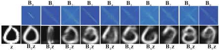
Figure 1: Top row: self-representation matrices Bk↪ k = 0↪ 1↪ ▷▷▷↪ 9 learned from the USPS database. Bottom row: a query sample (from class 0) and its reconstructed images Bkz↪ k = 0↪ 1↪ ▷▷▷↪ 9.
where I 2 <d⇥d is an identity matrix. Given a query sample z, its self-representation can then be computed as ˆ Bkz and the self-representation residual is e = z - ˆ Bkz.
For each class, we can learn its self-representation matrix as above, and then we have a set of K self-representation matrices, B1↪ ▷▷▷↪Bk↪ ▷▷▷↪BK (we omit the superscript " ˆ " for the convenience of expression). The query sample z can be represented by each of the matrices and the classification can be made by checking which class has the minimal selfrepresentation residual:
We call the above classifier self-representation induced classifier (SRIC).
We use an example to illustrate how SRIC works. As shown in Fig. 1, 10 self-representation matrices Bk↪ i = 0↪ 1↪ ▷▷▷↪ 9, are learned from handwritten digit dataset USPS [Hull, 1994]. Certainly, matrix Bk tends to represent better the features of sample from class k. Fig. 1 also shows a query sample z (from class 0) and the reconstructed samples Bkz by all Bk. We can see that z is well represented by B0 and it has the minimal self-representation residual on class 0, resulting in a correct classification.
2.3 Equivalence between SRIC and NSC
The NSC represents a sample from the perspective of sample similarity, while the proposed SRIC represents a sample from the perspective of feature similarity. Though the representation strategies are different, interestingly, it can be proved that they lead to the same classification result. We have the following theorem.
Theorem 1 SRIC is equivalent to l2-norm regularized nearest subspace classifier, i.e., Bk=Wk, k = 1↪ 2↪ ▷▷▷↪K.
Proof 1 Applying singular value decomposition to Xk, Xk = Uk⇤kVT k , where Uk 2 <d⇥d , ⇤k 2 <d⇥n and Vk 2 <n⇥n . Then Bk andWk becomes:
If d < n, we let ⇤k = [Hk 0], where Hk 2 <d⇥d . Then we have
Because Hk is a diagonal matrix, we have ⇤b = ⇤w. As Wk = Uk⇤wUTk and Bk = Uk⇤bUTk , we can get Bk =Wk.
have the same conclusion, i.e., ⇤b = ⇤w and Bk =Wk. If d = n, let ⇤k = Hk, ⇤b and ⇤w are the same as those ⇤b
and ⇤w when d < n. Hence, Bk = Wk also holds on when d = n.
From the above proof, we can have the following remark.
Remark 1 SRIC is equivalent to principal component analysis with shrinkage.
From the Proof, we can see that, Xk and Bk have the same set of eigenvectors, i.e., Uk. Denote the hth eigenvalue of Xk as σh, then the hth eigenvalue ⇤bh of Bk will be σ2h λ+σ2h . Therefore, for SIRC the eigenvalues of Bk will be shrunk to the range [0 1). The smaller the eigenvalue, the less the shrinkage ratio.
3 Discriminative self-representation induced classifier
3.1 Discriminative self-representation
The learning of self-representation matrix Bk in SRIC is rather generative but not discriminative since it only depends on the training data of class k. In light of the principle of self-representation in SRIC, we can then propose a discriminative self-representation induced classifier (DSRIC), which exploits the training data from all classes to learn Bk.
SRIC aims to learn a Bk such that the self-representation residual kXk -BkXkk2F could be minimized. However, SRIC does not take the samples of other classes into account. In order to make the classification more discriminative, we also expect that Bk cannot well represent the features of other classes. One may consider to maximize kXj -BkXjk2F , j 6= k while minimizing kXk -BkXkk2F . However, this will make the whole objective function non-convex. Another much easier but still very reasonable choice is to learn a Bk such that the self-representation of Xj , j 6= k, over it will approach to zero, i.e., kBkXjk2F is very small. In other words, Bk is discriminative to represent the features of class k but not other classes. With these considerations, we propose the following DSRICmodel to learn Bk:
where λ1 and λ2 are the regularization parameters.
In Eq. (12), the first term kXk -BkXkk2F aims to minimize the self-representation residual; the second term Pj6=k kBkXjk2F enforces that Xj↪ j 6= k will not be well represented by Bk; the last term regularizes Bk to make the solution more stable. It is apparent that we still have a closed form solution of Bk:
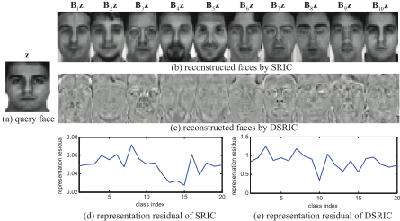
As shown in Fig. 2, we use a subset of AR database [Martinez, 1998] to show the difference between SRIC and DSRIC. Fig. 2(a) shows the query sample that belongs to subject 10. In Fig. 2(b), the query face z is well reconstructed by B10 learned by SRIC. However, from Fig. 2(d), we can see that z is misclassified to subject 15. The reconstructed faces using DSRIC are shown in Fig. 2(c). From Fig. 2(e), we can see that z is correctly classified to subject 10. Though the reconstruction ability of SRIC is superior to DSRIC, DSRIC has better discrimination ability than SRIC.
.
3.2 Classification and algorithms
After we get a set of matrices B1↪ B2↪ ▷▷▷↪ BK, a query sample z is classified to the class with the minimal reconstruction error.
The algorithm of DSRIC is shown in Algorithm 1.
Algorithm 1 The algorithm of discriminative selfrepresentation induced classifier (DSRIC)
Input: A query sample z and the training set X = [X1↪X2↪ ▷▷▷↪XK].
Output: label(z)
- 1: Calculate B1↪B2↪ ▷▷▷↪BK by Eq. (13);
- 2: Calculate rk = kz - Bkzk22 ;
- 3: Get label(z) = argmink¶rk♦.
3.3 Complexity analysis
In this section, we discuss the time and space complexity of SRIC, DSRIC.
Training complexity
SRIC and DSRIC need to learn K self-representation matrices in the training stage by Eq. (10) and Eq. (13), respectively. The time complexity to solve Eq. (10) and Eq. (13) is O(d3 ). Hence the training time complexity of SRIC and DSRIC is O(Kd3 ). During the training stage, all the methods should contain the training set. Hence, the training memory of SRIC and DSRIC is Kd2 + Kdn.
Testing complexity
In the testing stage, the time complexity of SRIC and DSRIC is O(Kd2 ). As DSRIC only needs to store a set of d ⇥ d matrices, the storage space of DSRIC is Kd2 . When the number of samples is much larger than the number of feature dimensions, the advantage of DSRIC in time complexity and storage consumption is quite significant.
We will compare SRIC and DSRIC with NNC [Cover and Hart, 1967], NSC [Chien and Wu, 2002], NAH [Vincent and Bengio, 2001], NCH [Vincent and Bengio, 2001], SRC [Wright et al., 2009], CRC [Zhang et al., 2011] and CROC [Chi and Porikli, 2014] in the experiments. The time and space complexity in the training and testing stages of all the methods are listed in Table 1.
| method | NNC | SRC | NSC | SRIC |
|---|---|---|---|---|
| Time(train) | / | / | O(Kn3 ) | O(Kd3 ) |
| Time(test) | O(Kdn) | O(d2 n" ) | O(Kdn) | O(Kd2 ) |
| Memory(train) | / | / | 2Kdn+n2 | Kd2 +Kdn |
| Memory(test) | Kdn | Kdn | 2Kdn | Kd2 |
| method | NCH | CRC | CROC | DSRIC |
| Time(train) | / | O((Kn)3 ) | O((Kn)3 +Kn3 | ) O(Kd3 ) |
| Time(test) | O((Kn)3 ) | O(Kdn) | O(Kdn) | O(Kd2 ) |
| Memory(train) | / | 2Kdn+ (Kn)2 | 3Kdn+ (Kn)2 | Kd2 +Kdn |
| Memory(test) | Kdn | 2Kdn | 3Kdn | Kd2 |
4 Experimental analysis
In this section, we test the performance of DSRIC 1 on eight UCI datasets, two handwritten digit recognition databases, two face recognition database and one gender classification dataset. We compare the proposed classifier with eight popular and state-of-the-art classifiers, including the nearest neighbor classifier (NNC) [Cover and Hart, 1967], nearest subspace classifier (NSC) [Chien and Wu, 2002], nearest convex hull classifier (NCH) [Vincent and Bengio, 2002], nearest affine hull classifier (NAH) [Vincent and Bengio, 2002], sparse representation based classifier (SRC) [Wright et al., 2009], collaborative representation based classifier (CRC) [Zhang et al., 2011] and collaborative representation optimization classifier (CROC) [Chi and Porikli, 2014]. Among them, NNC is a baseline benchmark, and the remaining are all representation based classifiers.
The performance of different classifiers is evaluated from three aspects: classification accuracy, the running time and memory consumption in the testing stage. In order to easily show the speedup and memory saving of DSRIC over other methods, in all the following experiments we take the running time and memory consumption of DSRIC as a unit (i.e., 1), and report the results of other methods based on it. All algorithms are run in an Intel(R) Core(TM) i7-2600K (3.4GHz) PC.
1 Since SRIC is equivalent to NSC, the results of SRIC will not be reported.
4.1 Parameter setting
There are two parameters in DSRIC: λ1 and λ2. In all the experiments, λ2 is fixed as 0.001 and λ1 is chosen on the training dataset by five-fold cross-validation. For the compared representation based methods, the parameters in NCH and NAH are set as 1 and 100, respectively, as suggested in the original paper; the regularization parameter in NSC, SRC and CRC is tuned from ¶0▷0005↪ 0▷001↪ 0▷005↪ 0▷01♦ and the best results are reported; following the experiment setting in [Chi and Porikli, 2014], the parameter of CROC is chosen by five-fold cross-validation on the training set.
4.2 UCI datasets
We first use eight datasets (derm, german, heart, hepatitis, iono, rice, thyroid, wdbc, wpbc, yeast) from the UCI machine learning repository [Asuncion and Newman, 2007] to evaluate the performance of DSRIC. The number of classes (c), number of features (f) and number of samples (s) of the eight datasets are illustrated in the right column of Table 2. The average classification accuracy(%), testing time (seconds) and testing memory (MB) over the eights datasets are listed at the bottom of Table 2.
From Table 2, we can see that the accuracy of DSRIC is about 2% higher than NSC, SRC and CRC, and 3% higher than CROC. Besides, DSRIC is much faster than the other representation based classifiers. Compared with NSC, SRC, CRC and CROC, the running time speedup by DSRIC is 64, 547, 106 and 130, respectively. Because NAH and NCH have to solve a QP problem for each query sample, the time consumption is very high compared with other classifiers. In terms of memory requirement, in this experiment DSRIC also has clear advantage.
| Database | NNC | SRC | NSC | NCH | NAH | CRC | CROC | DSRIC | c/f/s |
| derm | 96.1 | 97.1 | 97.4 | 96.5 | 96.9 | 97.1 | 97.7 | 97.6 | 6/34/366 |
|---|---|---|---|---|---|---|---|---|---|
| german | 68.8 | 74.1 | 70.6 | 70.6 | 71.3 | 72.9 | 72.9 | 73.4 | 2/20/1000 |
| heart | 76.7 | 83 | 78.1 | 76.3 | 76.5 | 84.1 | 83.3 | 83.7 | 2/13/270 |
| hepatitis | 82.5 | 86.8 | 86.8 | 82.1 | 81.7 | 84.7 | 86.7 | 87.5 | 2/19/155 |
| iono | 86.4 | 91 | 94.4 | 89.2 | 80.3 | 92.7 | 83.3 | 94.7 | 2/34/351 |
| rice | 80 | 82.9 | 84.7 | 80.7 | 80.5 | 83.8 | 82.9 | 86.6 | 2/5/104 |
| thyroid | 95.3 | 90.2 | 95.8 | 96.3 | 95.8 | 91.1 | 87.4 | 95.8 | 3/5/215 |
| wdbc | 95.4 | 93.5 | 92.3 | 94 | 93.9 | 94.7 | 95.3 | 95.6 | 2/30/569 |
| wpbc | 70.7 | 79.4 | 76.8 | 75.4 | 74.7 | 76.3 | 79.4 | 80.9 | 2/33/198 |
| yeast | 48.8 | 54.9 | 56.9 | 49.3 | 50.1 | 54.6 | 54.3 | 57.7 | 10/7/1484 |
| Accuracy | 80.1 | 83.3 | 83.4 | 81.0 | 80.2 | 83.2 | 82.3 | 85.4 | |
| Time | 2.8⇥104 | 547 | 64 | 4.9⇥105 | 6.6⇥105 | 106 | 130 | 1 | |
| Memory | 10.48 | 10.48 | 20.97 | 10.48 | 10.48 | 20.97 | 31.45 | 1 |
4.3 Handwritten digit recognition
USPS The USPS dataset contains 7,291 training and 2,007 testing images. Each class has about 650 training samples, and each handwritten digit sample is a 16⇥16 image. The experimental results are listed in Table 3. Since each class has enough training samples and the feature dimension is not high in this experiment, the simple NNC achieves the best accuracy. The recognition rate of DSRIC is only 0.3% lower than NNC. However, DSRIC is significantly faster than NNC with 10,000 times speedup. In addition, the memory consumption of NNC is 2.8 times larger than DSRIC.
| Method | NNC | SRC | NSC | NCH | NAH | CRC | CROC | DSRIC |
|---|---|---|---|---|---|---|---|---|
| Accuracy | 94.6 | 94.0 | 94.3 | 91.9 | 92.3 | 90.6 | 90.1 | 94.3 |
| Time | 1⇥104 | 1⇥104 | 165.6 | 5.1⇥104 | 7.7⇥104 | 150.8 | 977.1 | 1 |
| Memory | 2.848 | 2.848 | 5.696 | 2.848 | 2.848 | 5.696 | 8.544 | 1 |
MNIST The MNIST dataset includes a training set of 60,000 samples and a test set of 10,000 samples. The size of each image is 28⇥28 and there are 10 classes of digit images. Compared to USPS, there are more training samples. Table 4 lists the recognition rate, testing time and testing memory by different methods. Similar to the results in USPS, the recognition rate of DSRIC equals to NSC, and is 1.4% lower than NNC. However, DSRIC avoids the one-to-one searching process in the training set and is 18,000 faster than NNC, which is very important in real-time applications. Compared with SRC, DSRIC is 51 times faster and saves 7.65 times the memory. Please note that the performances of NCH, NAH, CRC and CROC are not reported because these methods need to process a 60,000⇥60,000 square matrix and out-of-memory in our PC.
| Method | NNC | SRC | NSC | NCH | NAH | CRC | CROC | DSRIC |
|---|---|---|---|---|---|---|---|---|
| Accuracy | 97.1 | 94.5 | 95.7 | / | / | / | / | 95.7 |
| Time | 1.8⇥104 | 6.3⇥104 | 649.3 | / | / | / | / | 1 |
| Memory | 7.653 | 7.653 | 15.306 | 7.653 | 7.653 | 15.306 | 22.959 | 1 |
4.4 Face recognition
LFW database The LFW database contains images of 5,749 subjects in unconstrained environment. LFW-a is a version of LFW after alignment using commercial face alignment software. We gathered the subjects which have no less than eleven samples and then formed a dataset with 136 subjects from LFW-a. Each face image is firstly cropped to 102⇥120 and then resized to 32⇥32 images. We select 9 face images per subject for training and use the remaining face images for testing.
The experimental results are shown in Table 5. DSRIC has the highest recognition accuracy. Since there are 158 subject and the feature dimension is 1024, DSRIC does not show advantages in memory in this experiment.
4.5 Gender classification
In this section, a non-occluded subset (14 images per subject) of the AR dataset is used. It includes face images of 50 male and 50 female subjects. The images from the first 25 males and 25 females are used for training and the remaining for testing. Following the experiment setting in [Zhang et al., 2011], each face image is cropped to 60⇥43 and PCA is used to reduce the feature dimension to 50. The classification accuracy, testing time and testing memory are given in Table 6. One can see that DSRIC achieves the highest accuracy, and it costs much less running time and memory than others.
| Method | NNC | SRC | NSC | NCH | NAH | CRC | CROC | DSRIC |
|---|---|---|---|---|---|---|---|---|
| Accuracy | 20.1 | 60.4 | 37.8 | 34.5 | 37.7 | 58.8 | 60.0 | 60.8 |
| Time | 14.7 | 25 | 0.55 | 80.2 | 107.9 | 0.77 | 1.28 | 1 |
| Memory | 0.009 | 0.009 | 0.018 | 0.009 | 0.009 | 0.018 | 0.026 | 1 |
| Method | NNC | SRC | NSC | NCH | NAH | CRC | CROC | DSRIC |
|---|---|---|---|---|---|---|---|---|
| Accuracy | 90.3 | 93.1 | 93.4 | 91.4 | 91.4 | 93.1 | 92.9 | 94.7 |
| Time | 1.4⇥104 | 8.4⇥103 | 44.4 | 2.5⇥105 | 3.6⇥105 | 41.1 | 92 | 1 |
| Memory | 7 | 7 | 14 | 7 | 7 | 14 | 21 | 1 |
5 Conclusions
In this paper we investigated the representation based classification problem from a "feature oriented" perspective. Different from the existing representation based classifiers that represent a sample as the linear combination of other samples, we explored to represent a feature by its relevant features in the data, which we call self-representation. A selfrepresentation induced classifier (SRIC) was then proposed, which learns a self-representation matrix per class and uses these matrices for classification. The query sample is then classified to the class with the minimal reconstruction error. We proved that SRIC is equivalent to nearest subspace classifier (NSC) with l2-norm regularization in terms of classification decision. Furthermore, it can be shown that SRIC is essentially the principal component analysis (PCA) with eigenvalue shrinkage. We then proposed a discriminative SRIC (DSRIC) classifier, which not only minimizes the feature selfrepresentation residual of this class but represents little the features of other classes. The time and space complexity of DSRIC (except for the training memory) is invariant to the number of training samples, which makes it very suitable for large scale datasets with many training samples, e.g., USPS and MNIST. Experimental results on different pattern recognition tasks showed that DSRIC achieves comparable or superior recognition rate to state-of-the-art representation based classifiers, while it has higher efficiency and lower memory consumption.
6 Acknowledgement
This work was supported by the National Program on Key Basic Research Project under Grant 2013CB329304, the National Natural Science Foundation of China under Grants 61502332, 61432011, 61222210.
@inproceedings{ijcai2016p348,
  title     = {A Self-Representation Induced Classifier},
  author    = {Zhu, Pengfei and Zhang, Lei and Zuo, Wangmeng and Feng, Xiangchu and Hu, Qinghua},
  booktitle = {Proceedings of the Twenty-Fifth International Joint Conference on
               Artificial Intelligence, {IJCAI-16}},
  publisher = {AAAI Press / International Joint Conferences on Artificial Intelligence},
  editor    = {Subbarao Kambhampati},
  pages     = {2442--2447},
  year      = {2016},
  month     = {7},
  url       = {https://ijcai.org/proceedings/2016/348},
}
TY - CPAPER TI - A Self-Representation Induced Classifier AU - Zhu, Pengfei AU - Zhang, Lei AU - Zuo, Wangmeng AU - Feng, Xiangchu AU - Hu, Qinghua T2 - Proceedings of the Twenty-Fifth International Joint Conference on Artificial Intelligence, IJCAI-16 PB - AAAI Press / International Joint Conferences on Artificial Intelligence PY - 2016 SP - 2442 EP - 2447 UR - https://ijcai.org/proceedings/2016/348 ER -Copied
Machine-readable versions of this paper, for tools and AI agents:





