
Household Structure Analysis via Hawkes Processes for Enhancing Energy Disaggregation
Proceedings of the Twenty-Fifth International Joint Conference on Artificial Intelligence. Pages 2553-2558.
Abstract
In energy conservation research, energy disaggregation becomes an increasingly critical task, which takes a whole home electricity signal and decomposes it into its component appliances. While householder's daily energy usage behavior acts as one powerful cue for breaking down the entire household's energy consumption, existing works rarely modeled it straightforwardly. Instead, they either ignored the influence between users' energy usage behaviors, or modeled the influence between the energy usages of appliances.With ambiguous appliance usage membership of householders, we find it difficult to appropriately model the influence between appliances, since such influence is determined by human behaviors in energy usage. To address this problem, we propose to model the influence between householders' energy usage behaviors directly through a novel probabilistic model, which combines topic models with the Hawkes processes. The proposed model simultaneously disaggregates the whole home electricity signal into each component appliance and infers the appliance usage membership of household members, and enables those two tasks mutually benefit each other. Experimental results on both synthetic data and four real world data sets demonstrate the effectiveness of our model, which outperforms state-of-the-art approaches in not only decomposing the entire consumed energy to each appliance in houses, but also the inference of household structures. We further analyze the inferred appliance-householder assignment and the corresponding influence within the appliance usage of each householder and across different householders, which provides insight into appealing human behavior patterns in appliance usage.
- [Baptista et al., 2014] M. Baptista, A. Fang, H. Prendinger, R. Prada, and Y. Yamaguchi. Accurate household occu- pant behavior modeling based on data mining techniques. In Proceedings of the Twenty-Eighth AAAI Conference on Artificial Intelligence, pages 1164-1170, 2014.
- [Barker et al., 2012] S. Barker, A. Mishra, D. Irwin, E. Cec- chet, P. Shenoy, and J. Albrecht. Smart*: An open data set and tools for enabling research in sustainable homes. In Proceedings of the 2012 Workshop on Data Mining Appli- cations in Sustainability, Beijing, China, 2012.
- [Blei and Jordan, 2005] D. Blei and M. Jordan. Variational inference for dirichlet process mixtures. In Bayesian Anal- ysis, volume 1, pages 121-144, 2005.
- [Blei et al., 2003] D. M. Blei, A. Y. Ng, and M. I. Jordan. Latent dirichlet allocation. J. Mach. Learn. Res., 3:993- 1022, March 2003.
- [C.-PenA et al., 2013] D. C.-PenA, M. Orozco-Alzate, and G. Castellanos-Dominguez. Selection of time-variant fea- tures for earthquake classification at the nevado-del-ruiz volcano. Comput. Geosci., 51:293-304, 2 2013.
- [Cox, 1972] D. R. Cox. Regression models and life-tables. Journal of the Royal Statistical Society. Series B (Method- ological), 34(2):pp. 187-220, 1972.
- [Darby, 2006] S. Darby. The effectiveness of feedback on energy consumption. Technical report, Environmental Change Institute, University of Oxford., 2006.
- [Dempster et al., 1977] A. P. Dempster, N. M. Laird, and D. B. Rubin. Maximum likelihood from incomplete data via the EM algorithm. Journal of the Royal Statistical So- ciety. Series B (Methodological), pages 1-38, 1977.
- [Errais et al., 2010] E. Errais, K. Giesecke, and L. R. Gold- berg. Affine point processes and portfolio credit risk. SIAM J. Fin. Math., 1(1):642-665, Sep 2010.
- [Hawkes, 1971] A. G. Hawkes. Spectra of some self-exciting and mutually exciting point processes. Biometrika, 58:83- 90, 1971.
- [Kolter and Jaakkola, 2012] J. Z. Kolter and T. Jaakkola. Ap- proximate inference in additive factorial hmms with appli- cation to energy disaggregation. In Proceedings of the Fif- teenth International Conference on Artificial Intelligence and Statistics, AISTATS 2012, La Palma, Canary Islands, April 21-23, 2012, pages 1472-1482, 2012.
- [Kolter and Johnson, 2011] J. Z. Kolter and M. J. Johnson. Redd: A public data set for energy disaggregation re- search. In Proceedings of the SustKDD workshop on Data Mining Applications in Sustainability, 2011.
- [Kolter et al., 2010] J. Z. Kolter, S. Batra, and A. Y. Ng. Energy disaggregation via discriminative sparse coding. In Advances in Neural Information Processing Systems, pages 1153-1161, 2010.
- [Li and Zha, 2014] L. Li and H. Zha. Learning parametric models for social infectivity in multi-dimensional hawkes processes. In AAAI Conference on Artificial Intelligence, 2014.
- [Li and Zha, 2015] L. Li and H. Zha. Energy usage behav- ior modeling in energy disaggregation via marked hawkes process. In AAAI Conference on Artificial Intelligence, 2015.
- [Li et al., 2014] L. Li, H. Deng, A. Dong, Y. Chang, and H. Zha. Identifying and labeling search tasks via query- based hawkes processes. In Proceedings of the 20th ACM SIGKDD International Conference on Knowledge Discov- ery and Data Mining, KDD '14, pages 731-740, New York, NY, USA, 2014. ACM.
- [Mendez et al., 2010] M. O. Mendez, M. Matteucci, V. Cas- tronovo, L. F. Strambi, S. Cerutti, and A. M. Bianchi. Sleep staging from heart rate variability: time-varying spectral features and hidden markov models. International Journal of Biomedical Engineering and Technology, 3, 1 2010.
- [Neenan and Robinson, 2009] B. Neenan and J. Robinson. Residential electricity use feedback: A research synthe- sis and economic framework. Technical report, Electric Power Research Institute., 2009.
- [Ogata, 1988] Y. Ogata. Statistical models for earthquake oc- currences and residual analysis for point processes. Jour- nal of the American Statistical Association., 83(401):9-27, 1988.
- [Parson et al., 2012] O. Parson, S. Ghosh, M. Weal, and A. Rogers. Non-intrusive load monitoring using prior models of general appliance types. In Proceedings of the Twenty-Eighth AAAI Conference on Artificial Intelligence, July 22 -26, 2012, Toronto, Canada, pages 356-362, 2012.
- [Perry and Wolfe, 2013] P. O. Perry and P. J. Wolfe. Point process modeling for directed interaction networks. In Journal of the Royal Statistical Society, 2013.
- [Schoenberg, 2010] F.P. Schoenberg. Introduction to point processes. Wiley Encyclopedia of Operations Research and Management Science, pages 616-617, 2010.
- [Shao et al., 2013] H. Shao, M. Marwah, and N. Ramakr- ishnan. A temporal motif mining approach to unsuper- vised energy disaggregation: Applications to residential and commercial buildings. In AAAI Conference on Arti- ficial Intelligence, 2013.
- [Stomakhin et al., 2011] A. Stomakhin, M. B. Short, and A. L. Bertozzi. Reconstruction of missing data in social networks based on temporal patterns of interactions. In- verse Problems., 27(11), Nov 2011.
- [Swan and Allan, 1999] R. Swan and J. Allan. Extracting significant time varying features from text. In Proceedings of the Eighth International Conference on Information and Knowledge Management, CIKM '99, pages 38-45, New York, NY, USA, 1999. ACM.
- [Wytock and Kolter, 2014] M. Wytock and J. Z. Kolter. Con- textually supervised source separation with application to energy disaggregation. In Proceedings of the Twenty- Eighth AAAI Conference on Artificial Intelligence, pages 486-492, 2014.
References were extracted automatically from the PDF and may contain errors.
Full text extracted automatically from the PDF; figures, tables and equations may differ. The PDF is the version of record.
1 Introduction
One critical data analysis issue in modern society is energy conservation, which encourages the exploration of energy usage behaviors in households. Energy disaggregation - the task of taking a whole-house energy signal and separating it into its component appliances, is an important task in this area, since existing studies [Darby, 2006; Neenan and Robinson, 2009; Wytock and Kolter, 2014; Shao et al., 2013] claimed that household members pay more attention to energy conservation if they're shown breakdown energy consumption records, especially the records of appliance usage behaviors of each householder. However, the collection of such fine-grained energy consumption data requires numerous additional monitoring hardware. Nowadays, a limited number of families are equipped with smart-grid devices, which are only able to record the energy consumption for each appliance, rather than the householder who uses it. While several energy disaggregation methods have been proposed to obtain the first type of fine-grained records, few of them studied the corresponding household structures, which can provide us the record of appliance usage membership of householders. We notice that those two tasks are closely related as their underlying key cues are the same - householder's behavior in energy usage [Baptista et al., 2014], which can include: how users perform their daily routines, how they share the usage of appliances, and users' habits in using certain types of appliances. Thus we explore solutions that simultaneously address those two tasks, based on the modeling of energy usage behaviors of householders.
⇤ Part of the work is supported by NIH R01 GM108341 and STCSM 15JC1401700.
Despite of the importance of understanding householders' energy usage behaviors, existing works on energy disaggregation rarely modeled them directly. Those works mostly focused on the distribution of energy consumption of each appliance alone [Kolter et al., 2010; Kolter and Jaakkola, 2012; Parson et al., 2012]. They either learned the energy usage patterns of each appliance within a certain period (for instance, a week), or studied the relationship between energy usage patterns across adjacent time slots. One critical cue in understanding householders' energy usage behaviors is the influence in between, i.e., whether and how much a householder's current appliance usage motivates his/her or other people's usage of certain appliances in the future. Appropriate modeling of the influence between householders' energy usage behaviors enables an accurate inference of the energy usage at each time slot, thus benefits the disaggregation of the energy consumption in each time slot into different appliances. The major challenge in such influence modeling is that, the state-of-the-art smart-grid data rarely records the number of household members, and the exact timestamp when a certain member uses a certain appliance. Recent studies attempted to capture the relationship between the energy usages of different appliances instead, since the energy consumption of each appliance is determined by the user behavior. Those works expected such relationship will be able to reveal the influence between the energy usage behaviors of different users in the same household across different time slots. However, with ambiguous appliance usage membership of householders, it is difficult to infer such relationship appropriately and explain reasonably.
To this end, we propose a novel probabilistic model that combines the Hawkes processes with topic models. This model is designed to simultaneously infer the appliance usage membership of household members and disaggregate the whole home electricity signal into each component appliance. In the proposed model, the topic model part models the distribution of the appliance usage of householders, designed to infer the appliance usage membership of householders in each time slot, while the Hawkes process part models the occurrences of observed events, and captures the influence between the energy usage behaviors from the same or between different householders across different time slots.
In a nutshell, our major contributions include: 1) We make use of the temporal and energy amount information in solving both the energy disaggregation and household structure analysis task, based on the exploration of householders' daily routines in energy consumption; 2) We directly model the influence between energy usage behaviors from different householders across different time slots, which many existing works failed to model; 3) We propose a novel probabilistic model that combines the Hawkes processes with topic models, which is able to solve the above two tasks simultaneously, and makes them mutually benefit each other.
2 ProblemDefinition
Let us look into an energy consumption scenario that contains M houses. In each house, a number of C appliances are used in a sequence of N time slots T = ¶tn↪ n = 1↪ ▷ ▷ ▷ ↪ N♦. Notice that multiple appliances may be used side by side in the same time slot, while one appliance is not necessarily always in use.
On one hand, in the task of energy disaggregation, we only observe the total amount of consumed energy Xm↪n in each time slot n in house m, while the amount of consumed energy xm↪n↪a of each appliance a used in that time slot is not available. The target of energy disaggregation is to predict each xm↪n↪a based on the observed T and X. Since the exact amount of xm↪n↪a is difficult to be predicted from Xm↪n directly, we assume each appliance has L energy consumption levels (with the amount from low to high), and introduce a set of latent variables ¶Ym↪n↪a↪l♦ to denote whether the a-th appliance is used at level l in the n-th time slot in house m, along with the consumption level of each appliance ✓a↪l.
On the other hand, in the task of household structure analysis, we are to learn the number of household members in each family and each appliance's usage membership of householders, which we denote using a set of latent variables Z. For each Ym↪n↪a↪l = 1, which denotes one occurrence of appliance usages in a single time slot, we have a corresponding Zm↪n↪a↪l that indicates the corresponding householder membership, i.e., which householder uses the appliance a at level l in the n-th time slot within house m. Next we show how the tasks of energy disaggregation and household structure inference can be addressed simultaneously and mutually benefit each other in a unified model.
2.1 LDA in Household Structure Inference
In the exploration of the household structure of each family in the smart-grid data, the key idea is that each householder performs a certain type of appliance usage pattern in his/her daily routine, and our task is to cluster householders based on their appliance usage patterns. One popular solution for clustering problems is graphical models like LDA [Blei et al., 2003], which has been proven to be effective in topic discovery by clustering words that co-occur in the same document into topics. Let us first introduce how to use LDA to detect appliance usage patterns given inferred Y . One straightforward idea is to treat each family as a document, and cluster appliance usages (as words in document clustering) that co-occur in the same family into topics, since appliance usages of householders from the same family are more likely to follow the same pattern than those of householders from different families. Notice that under such circumstances, each topic/pattern 'k is actually the distribution of appliance usages. Our LDA model assumes K patterns lie in the observed smart-grid data, and each family m is associated with a randomly drawn vector ⇡m, where ⇡m↪k denotes the probability that a householder from family m performs appliance usage pattern k. If an appliance a is used in energy consumption level l in the n-th time slot in the daily routine of family m, i.e., Ym↪n↪a↪l = 1, a K-dimensional binary vector Zm↪n↪a↪l = [ym↪n↪a↪l↪1↪ ▷ ▷ ▷ ↪ ym↪n↪a↪l↪K]T is used to denote the appliance's usage pattern membership.
2.2 Parametric Hawkes Processes
The multi-dimensional Hawkes process is a class of selfor mutually-exciting point process models [Hawkes, 1971], which are widely used to describe data that are localized at a finite set of time points ¶t1↪ ▷ ▷ ▷ ↪ tN♦ [Schoenberg, 2010]. Formally, the multi-dimensional Hawkes process on an event cascade ¶tl♦Nl=1 is defined to be a M-dimensional point process with the intensity of the m-th dimension given by:
Here θm denotes the base intensity of the m-th dimension, (t - tl) is a time-decaying kernel, while ↵m↪m0 denotes the infectivity from events in the m-th dimension to events in the m0 -th dimension. Hawkes process has been widely used in applications, such as earthquake prediction [Ogata, 1988], sales modeling [Errais et al., 2010], crime modeling [Stomakhin et al., 2011], and information retrieval [Li et al., 2014].
In many real world social networks, ↵'s are not independent from each other, and may vary with respect to time. Under such scenarios, learning one separate ↵ for each pair of dimensions (m↪m0 ) becomes inappropriate. Instead, recent work [Li and Zha, 2014] decomposed each ↵ into a linear combination of K time-varying features as:
| Pattern p | Description |
|---|---|
| a | the historical usage of appliance a |
| a&a0 | the historical usage of appliance a0 before using appliance a |
| (a↪ k) | the historical usage of appliance a of householder k |
| (a&a0 ↪ k) | the historical usage of appliance a0 of house- holder k before using appliance a |
| (al) | the historical usage of appliance a at level l |
| (al&a0l0 ↪ k) | the historical usage of appliance a0 at level l0 of householder k before using appliance a at level l |
where β is the vector of coefficients that we are to learn instead of ↵. xm↪m0(t) is a time-varying dyad-dependent vector, which is supposed to reflect some kind of relationship between dimension m and m0 .
In the application of energy disaggregation, the event we are to model is the usage of an appliance at a certain level in a time slot. Under such scenario, the dimension m of an event is the pair of appliance and its usage level (a↪ l). Thus, the intensity of the usage of appliance a at level l in time slot t can be formulated as:
Time-varying Features based on Household Structures
Time-varying features [Swan and Allan, 1999] attract ever increasing attentions in analyzing temporal data, such as email communication [Perry and Wolfe, 2013], seismic events [C.- PenA et al., 2013], and Heart Rate Variability (HRV) signals [Mendez et al., 2010]. These features usually vary with respect to time, and count the number of appearances of a certain pattern involving one individual or one individual-pair in a certain time range formulated as:
where p represents a certain defined pattern, [t - ∆t↪ t) is the time interval from some ancient timestamp to the current timestamp.
Table 1 shows several patterns we adopt in this paper. Our feature design is inspired by the features proposed in [Perry and Wolfe, 2013]. The novelty of our design is that we propose features in more general forms, and also explore brand-new patterns in networks (the household structure in our problem), thus producing far more features.
As shown in Table 1, our features are generally designed to measure the appliance usage history related to a certain appliance and a certain pair of appliances, and imply how a householder's historical appliance usages influence the current appliance usage of him/her or other householders in the same family. Based on above collected features, we are able to form a length-V feature vector xa↪l(t↪ Z) for the appliance a with consumption level l used at timestamp t through:
where Pa↪l↪a0 ↪l0(Z) refers to the set of patterns that involves both appliance a (at level l) and appliance a0 (at level l0 ) listed as in Table 1, based on the current inferred appliance usage membership of householders Z. Thus for each timestamp t, we have a unique set of feature vectors ¶xa↪l↪a0 ↪l0 (t↪ Z)♦ utilized in intensity function λ(t).
In our tasks, building a parametric Hawkes processes on Y relates Ym↪n↪a↪l, the inference of a-th appliance usage state l in the n-th time slot in house m, with those of other appliances in different time slots, thus can be expected to sharply raise the inference accuracy.
2.3 ParaHawkes-LDA
According to the above description of the inference of householder structure and the prediction of energy disaggregation, we find that the inference of Y and Z depends on each other as the observed data. Thus we can propose a novel probabilistic model that combines the LDA model with the parametric Hawkes process to make them mutually benefit each other in solving the above two tasks side by side.
The generative model produces the entire energy consumption as follows:
- For each appliance a,
- draw a L dimensional vector ✓a, in which each dimension indicates a single energy consumption level of the appliance.
- For each family m,
- draw a K dimensional membership vector ⇡m ⇠ Dirichlet(↵).
- For the n-th time slot,
- For the a-th appliance,
- draw whether it will be used by Ym↪n↪a↪l ⇠ ParaHawkes(λ(·)), where the intensity λ is defined as in Eqn (3);
- draw the amount of consumed energy of device xm↪n↪a ⇠ Pl Ym↪n↪a↪lGaussian(✓a↪l↪ σ); 1
Note that in our ParaHawkes-LDA model, the number of appliances used in the same time slot is constrained by the total amount of consumed energy at that time. Such constraints not only benefit the inference of appliance usage patterns of householders, but also enable the modeling of multiple events that occur in the same time slot, which most existing Hawkes processes failed to handle.
- Calculate the total amount of consumed energy in the n-th time slot Xm↪n = Pa xm↪n↪a.
Under our ParaHawkes-LDA model, the joint probability of data T = ¶N(·)♦ = ¶¶tn♦Nn=1 ♦, X = ¶¶Xn♦Nn=1 ♦ and latent variables ⇡, Y , Z can be written as follows:
1 In our experiments, we use a constant σ.
2.4 Inference
In this section, we describe the inference algorithm for our proposed model. Since the latent variables Y for solving the energy disaggregation task and Z for solving the household structure analysis task mutually depend on each other as the respective input, we adopt a coordinate descent framework and update each set of latent variables alternatively.
Under ParaHawkes-LDA model, given observations of both temporal information T and consumed energy X of energy consumption event sequences, the log-likelihood for the complete data is given by log p(T↪X♣↵↪ ✓↪ '↪ θ↪ !). Since this true posterior is hard to infer directly, we turn to variational methods [Blei and Jordan, 2005], which posits a distribution over the latent variables to make it close to the true posterior in Kullback-Leibler (KL) divergence.
where q1 is a Dirichlet, q2 is a multinomial, and ¶γ1:M↪ Φ↪ ⇢♦ are the set of variational parameters. We optimize those free parameters to tight the following lower bound L0 for our likelihood:
Under a coordinate descent framework, we optimize the lower bound as in Eqn (4) against each latent variable, and obtain the update rule for the variational variable φ corresponding to appliance usage states as:
And the update rule for the variational variable ⇢ corresponding to appliance usage membership of householders is:
To learn the parameters in the proposed ParaHawkes-LDA model, we use a variational expectation-maximization (EM) algorithm [Dempster et al., 1977]. This variational EM algorithm optimizes the lower bound as in Eqn (4) instead of the real likelihood, it iteratively approximates the posterior by fitting the variational distribution q and optimizes the corresponding bound against the parameters.
To update ↵, we use a Newton-Raphson method, since the approximate maximum likelihood estimate of ↵ doesn't have a closed form solution. The Newton-Raphson method is conducted with a gradient and Hessian as follows:
The learning of base intensity θ and coefficients β in the part of parametric Hawkes model are performed based on the equations introduced in [Li and Zha, 2014].
In our mean-field variation inference algorithm, the computational cost of inferring variational variables is O(MNC 2L2KV ), where V is the length of the feature vector x. The computational cost of the estimation of Hawkes hyper-parameters is O(MN 2C 2L2V ), which can be reduced to O(MNC 2L2V ) by only considering the influence in temporally-close time slots. Thus the total computational cost of our algorithm is O(MNC 2L2KV ). Since in realworld scenario, influence exists only among limited pair of appliances and patterns, C 2L2 can be reduced to some much smaller constant. Furthermore, the number of appliance usage patterns K and the feature vector size V is under the control of our model, which can be also very small, thus the above cost can be viewed as linear in the number of events.
3 Experiments
We evaluated our ParaHawkes-LDA model on both synthetic and real-world data sets, and compared the performance with the following baselines:
Cox: This is a normal Cox proportional hazards model that influence between the occurrences of events only without the inference of household structure [Cox, 1972];
M-Hawkes: This is a marked Hawkes process that is able to capture the influence from the occurrence and the marks of one energy usage event to the occurrence and the marks of subsequent usage events in the future [Li and Zha, 2015];
AFAMAP: This is an approximation inference algorithm, named Additive Factorial Approximate MAP, to efficiently solve the additive factorial hidden Markov model by looking at the observed difference in consumed energy, and incorporating a robust mixture component that can account for unmodeled observation [Kolter and Jaakkola, 2012];
NIALM: This method, named non-intrusive load monitoring, iteratively separates individual appliances from an aggregate energy consumption record, and turns prior models of general appliance types for each appliance [Parson et al., 2012].
3.1 Synthetic data
Data Generation. Given parameters (M↪N↪K↪C↪ L↪ V↪ ↵↪ ✓↪ '↪ θ↪ !), the synthetic data is sampled according to the proposed generative model. Here each element in θ and ! are randomly generated in [0▷5ˆθ↪ 1▷5ˆθ] and [0▷5ˆ!↪ 1▷5ˆ!] respectively before the simulation. In addition, ↵ is a vector of size K, where the element ↵k is generated in [0▷5ˆ↵↪ 1▷5ˆ↵]. Our synthetic data are simulated with two different settings:
- Small: M = 10, N = 100, K = 3, C = 10, L = 3, V = 20, ˆθ = 0▷01, ˆ! = 0▷5, ˆ↵ = 0▷1, ˆ ✓ = 10. Simulations were run 1,000 times using the pre-generated parameters θ, !;
- Large: M = 100, N = 9,000, K = 5, C = 50, L = 3, V = 100, ˆθ = 0▷01, ˆ! = 0▷5, ˆ↵ = 0▷1, ˆ ✓ = 10. Simulations were run 10 times.
To test the robustness of our method, we add two types of noise to the original synthetic data:
Event Noisy: We generate additional 10% of total number of events randomly in the time window of each already sampled event sequence, and add them to the sequence;
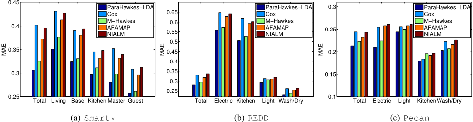
Table 2: Inference and Estimation of ParaHawkes-LDA
| Data set | MAE(θ) | MAE(!) | MAE(Y ) | MAE(Z) |
|---|---|---|---|---|
| S-Synthetic | 0.047 | 0.183 | 0.140 | 0.224 |
| S-E-Noisy | 0.067 | 0.261 | 0.152 | 0.273 |
| S-M-Noisy | 0.083 | 0.287 | 0.166 | 0.322 |
| L-Synthetic | 0.121 | 0.323 | 0.195 | 0.239 |
| L-E-Noisy | 0.134 | 0.332 | 0.226 | 0.311 |
| L-M-Noisy | 0.143 | 0.356 | 0.261 | 0.365 |
| Data set | PHawkes-L | Cox | M-Hawkes | AFAMAP | NIALM |
|---|---|---|---|---|---|
| S-Synthetic | -85.13 | -98.74 | -90.92 | -100.25 | -103.38 |
| S-E-Noisy | -95.08 | -106.86 | -101.53 | -109.76 | -114.52 |
| S-M-Noisy | -100.31 | -121.42 | -108.06 | -122.48 | -122.89 |
| L-Synthetic | -134.18 | -159.39 | -149.94 | -162.85 | -169.08 |
| L-E-Noisy | -144.82 | -172.71 | -162.01 | -176.69 | -181.43 |
| L-M-Noisy | -150.17 | -178.68 | -168.39 | -182.15 | -186.71 |
| Smart* | -142.03 | -163.48 | -145.39 | -157.83 | -160.35 |
| Pecan | -188.82 | -221.05 | -192.17 | -209.12 | -216.43 |
| REDD | -167.89 | -191.73 | -171.37 | -182.37 | -187.51 |
In this table, PHawkes-L stands for ParaHawkes-LDA.
Mark Noisy: Instead of using the simulatedXn as the consumed energy at the n-th time slot, we use a noisy value X0n which is obtained by adding Guassian noise on Xn:
The default value of σ0 is set to be 1.
Inference and Estimation. Table 2 evaluates both the accuracy of our proposed variational inference algorithm in parameter estimation and latent variable inference on the synthetic data. We find that, on the small synthetic data, ParaHawkes-LDA can recover the Hawkes parameters θ and ! very well, and accurately estimate the LDA hyperparameters ↵. On the large synthetic data, ParaHawkesLDA's performance on parameter estimation becomes worse. The sharply increased number of appliances makes the event occurrence prediction more difficult, and further affects the learning of users' energy usage behavior patterns. On both noisy data sets, the performance of ParaHawkes-LDA become worse.
3.2 Real-world Data
We also conducted extensive experiments on four real-world data sets. The first data set is Smart* [Barker et al., 2012], which is a high-resolution data set from three homes including over 50 appliances. The second data set is Reference Energy Disaggregation Dataset (REDD) [Kolter and Johnson, 2011]. This data set comprises six houses, for which both household aggregate and circuit-level power demand data are collected. The third data set is Pecan Street 2 . This data set collects one-minute resolution disaggregated data for 450+ homes, dating from late 2012 to late 2014. Meanwhile, this data set also records the number of householders in each home, thus can also be used to justify the performance of household structure inference. The fourth data set is a Irish smart-grid data set collected by Commission for Energy Regulation (CER) 3 . This data set collects energy data from over 4000 homes, but only records the total amount of consumed energy of a house in each time slot, and lacks the groundtruth information of the amount of disaggregated energy of each appliance, thus unable to be used for the evaluation of the performance of energy disaggregation. However, this data set records the number of household membership, thus we use it to evaluate the performance on household structure analysis in addition.
2 http://www.pecanstreet.org/
3 http://www.cer.ie/
Model Fitness. Table 3 shows the log predictive likelihood on energy consumption falling in the final 10% of the total time of data. To avoid overfitting issues, we adopt a k-fold cross validation strategy, and select the optimal number of user appliance usage pattern K. In Table 3, ParaHawkesLDA fits both synthetic and real-world data significantly better than alternative probabilistic models, which illustrates the importance of exploring household structure in smart-grid data. The comparison on synthetic data is meaningful since we add noise into it. On both noisy data sets, the performances of all models become worse. However, the decrease of the performance of ParaHawkes-LDA is smaller than baselines, which demonstrates the robustness of our proposed model. Thus when the usage timestamps and the amounts of consumed energy of some appliances are misrecorded, ParaHawkes-LDA performs better in energy disaggregation, and learns householders' appliance usage behaviors better.
Performance on Energy Disaggregation. To illustrate the effectiveness of the proposed model in energy disaggregation, we compare it with all baselines measured by MAE(X), i.e., the mean absolute error between the ground-truth consumed energy of each appliance x and the estimated consumed energy ˆx. According to Figure 1, ParaHawkes-LDA not only outperforms all compared methods in general, but also gains a better performance than competing methods on all categorized appliances. Such results demonstrate the importance of inferring the household structure in smart-grid data. In particular, the advantage of the proposed model over M-Hawkes shows that modeling the influence between the appliance usage behaviors of householders straightforwardly is more appropriate than vaguely modeling the influence between the energy usages of appliances without considering the participation of householders. M-Hawkes performs better than the rest baselines, which emphasizes the importance of modeling influence between the appliance usage behaviors.
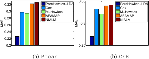
Performance on Household Structure Analysis. We evaluate the performance of household structure analysis by the mean absolute error (MAE) of the number of householders in each house. For each house m, the proposed model estimates an optimal householder number based on the inferred pattern distribution ⇡m, and compare it with the ground-truth number. Here we choose MAE as the metric since the structures of houses with a large number of members are more difficult to analyze. Moreover, since all alternative models for energy disaggregation are unable to infer the household structure, in this series of experiments, we use those models in a two-step framework that 1) first disaggregates the consumed energy into each appliance, and then 2) employ the LDA model to infer the household structure according to the disaggregated results of energy consumption. According to Figure 2, ParaHawkes-LDA performs at least 7% better than all compared methods on both real-world data sets, which illustrates the effectiveness of the proposed model in analyzing household structures along with addressing energy disaggregation. We also notice that using the parametric Hawkes model and the LDA model in a two-step framework results in a much worse performance than the proposed model, which highlights the mutual benefit of those two parts when combined into a unified model.
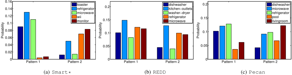
Appliance Usage Patterns of Householders. Based on the appliance distribution parameters ' of appliance usage patterns learned by the proposed model, we analyze the appliance usage patterns of householders detected in real world smart-grid data. According to Figure 3, the appliance usage preferences in different patterns are very different from each other. The results in the Smart* data highlight the difference between the type of householder who is busy with housework and the type of householder who enjoys work and games through IT devices. The REDD data mainly records the energy usage in kitchen. However, we can still tell the difference between housework people and people who use kitchen mainly for self-feeding. In Pecan, the difference of appliance usage distribution between housework people and nonhousework people is also very significant. The latter group of people use pool and living rooms for fun more frequently.
4 Conclusion and FutureWork
In this paper, we propose to solve the tasks of energy disaggregation and household structure analysis simultaneously and make them mutually benefit each other. Our paper presented a probabilistic model that integrates the LDA with the parametric Hawkes process to capture the influence between the appliance usage behaviors of householders in the same family. In future work, it would be interesting to consider additional features that capture the influence between the energy usage behaviors of householders.
@inproceedings{ijcai2016p363,
  title     = {Household Structure Analysis via Hawkes Processes for Enhancing Energy Disaggregation},
  author    = {Li, Liangda and Zha, Hongyuan},
  booktitle = {Proceedings of the Twenty-Fifth International Joint Conference on
               Artificial Intelligence, {IJCAI-16}},
  publisher = {AAAI Press / International Joint Conferences on Artificial Intelligence},
  editor    = {Subbarao Kambhampati},
  pages     = {2553--2558},
  year      = {2016},
  month     = {7},
  url       = {https://ijcai.org/proceedings/2016/363},
}
TY - CPAPER TI - Household Structure Analysis via Hawkes Processes for Enhancing Energy Disaggregation AU - Li, Liangda AU - Zha, Hongyuan T2 - Proceedings of the Twenty-Fifth International Joint Conference on Artificial Intelligence, IJCAI-16 PB - AAAI Press / International Joint Conferences on Artificial Intelligence PY - 2016 SP - 2553 EP - 2558 UR - https://ijcai.org/proceedings/2016/363 ER -Copied
Machine-readable versions of this paper, for tools and AI agents:





