
ST-MVL: Filling Missing Values in Geo-Sensory Time Series Data
Proceedings of the Twenty-Fifth International Joint Conference on Artificial Intelligence. Pages 2704-2709.
Abstract
Many sensors have been deployed in the physical world, generating massive geo-tagged time series data. In reality, we usually lose readings of sensors at some unexpected moments because of sensor or communication errors. Those missing readings do not only affect real-time monitoring but also compromise the performance of further data analysis. In this paper, we propose a spatio-temporal multi-view-based learning (ST-MVL) method to collectively fill missing readings in a collection of geo-sensory time series data, considering 1) the temporal correlation between readings at different timestamps in the same series and 2) the spatial correlation between different time series. Our method combines empirical statistic models, consisting of Inverse Distance Weighting and Simple Exponential Smoothing, with data-driven algorithms, comprised of User-based and Item-based Collaborative Filtering. The former models handle the general missing cases based on empirical assumptions derived from history data over a long period, standing for two global views from a spatial and temporal perspective respectively. The latter algorithms deal with special cases where empirical assumptions may not hold, based on recent contexts of data, denoting two local views from a spatial and temporal perspective respectively. The predictions of the four views are aggregated to a final value in a multi-view learning algorithm. We evaluate our method based on Beijing air quality and meteorological data, finding our model's advantages beyond ten baseline approaches.
- [Antti et al., 2010] Sorjamaa Antti, Lendasse Amaury, Cornet Yves, Deleersnijder. An improved methodology for filling missing values in spatiotemporal climate data set. Computational Geosciences, 14(1):55-64, 2010.
- [Chen and Liu, 2012] Feng-Wen Chen, and Chen-Wuing Liu. Estimation of the spatial rainfall distribution using inverse distance weighting in the middle of Taiwan. Paddy and Water Environment, 10(3):209-222, 2015.
- [Ceylan et al., 2013] Yozgatligil Ceylan, Sipan Aslan, Cem Iyigun, and Inci Batmaz. Comparison of missing value imputation methods in time series: the case of Turkish meteorological data. Theoretical and applied climatology 112(1):143-167, 2013.
- [Gardner, 2006] Everette S. Gardner. Exponential smoothing: The state of the art -Part II. International journal of forecasting, 22(4):637-666, 2006.
- [George and Wong, 2008] George Y. Lu, and David W. Wong. An adaptive inverse-distance weighting spatial interpolation technique. Computers & Geosciences, 34(9):1044-1055, 2008.
- [Fung, 2006] David Sheung Chi Fung. Methods for the estimation of missing values in time series. Doctoral dissertation, Edith Cowan University Perth, 2006.
- [Gruenwald et al., 2010] Le Gruenwald, Md Shiblee Sadik, Rahul Shukla, and Hanqing Yang. DEMS: a data mining based technique to handle missing data in mobile sensor network applications. In Proceedings of the 7th Interna- tional Workshop on Data Management for Sensor Net- works, pages 26-32, 2010.
- [Johan at el., 2014] Lindström Johan, Adam A. Szpiro, Paul D. Sampson, Assaf P. Oron, Mark Richards, Tim V. Larson, and Lianne Sheppard. A flexible spatio-temporal model for air pollution with spatial and spatio-temporal covariates. Environmental and ecological statistics, 21(3):411-433, 2014.
- [Lawson and Hanson, 1974] Charles L. Lawson, and Richard J. Hanson. Solving least squares problems. Englewood Cliffs, NJ: Prentice-hall, 161, 1974.
- [Lee et al., 2008] Dongheui Lee, Kulic Dana, and Nakamura Yoshihiko. Missing motion data recovery using factorial hidden markov models. 2008. In Proceedings of the 12th International Conference on Robotics and Automation, papes 1722-1728, 2008.
- [Little and Rubin, 2014] Roderick JA Little, and Donald B. Rubin. Statistical analysis with missing data. John Wiley & Sons, 2014.
- [Li and Parker, 2014] YuanYuan Li, and Lynne E. Parker. Nearest neighbor imputation using spatial-temporal corre- lations in wireless sensor networks. Information Fusion, 15:64-79, 2014.
- [Ma et al., 2007] Hao Ma, Irwin King, and R. Lyu Michael. Effective missing data prediction for collaborative filter- ing. In Proceedings of the 30th International Conference on Research and Development in Information Retrieval, pages 39-46, 2007.
- [Pan and Li, 2010] Liqiang Pan, and Jianzhong Li. K-Nearest Neighbor Based Missing Data Estimation algorithm in wireless sensor networks. Wireless Sensor Network, 2(02):115, 2010.
- [Sarwar et al., 2001] Badrul Sarwar, George Karypis, Joseph Konstan, and John Riedl. Item-based collaborative filt- ering recommendation algorithms. In Proceedings of the 10th International Conference on World Wide Web, pages 285-295, 2001.
- [Sorjamaa and Amaury, 2007] Antti Sorjamaa, and Lendasse Amaury. Time series prediction as a problem of missing values. In Proceedings of the 17th International Joint Conference on Neural Networks, pages 2948-2953, 2007.
- [Silva-Ramírez et al., 2011] Esther-Lydia Silva-Ramírez, Pino-Mejías Rafael, López-Coello Manuel, and Cubiles- de-la-Vega María-Dolores. Missing value imputation on missing completely at random data using multilayer perc- eptrons. Neural Networks, 24(1):121-129, 2011.
- [Su and Khoshgoftaar, 2009] Xiaoyuan Su, and Taghi M. Khoshgoftaar. A survey of collaborative filtering techni- ques. Advances in Artificial Intelligence, 4, 2009.
- [Tobler, 1970] Waldo R. Tobler. A computer movie simu- lating urban growth in the Detroit region. Economic Geography, 46(2):234-240, 1970.
- [Wang et al., 2006] Jun Wang, Arjen P. De Vries, and Marcel JT Reinders. Unifying user-based and item-based collabo- rative filtering approaches by similarity fusion. In Procee- dings of the 29th International ACM SIGIR Conference on Research and Development in Information Retrieval, pages 501-508, 2006.
- [Wu and Li, 2013] Tingting Wu, and Yingru Li. Spatial inter- polation of temperature in the United States using residual kriging. Applied Geography, 44:112-120, 2013.
- [Zheng, 2015] Yu Zheng. Methodologies for cross-domain data fusion: an overview. IEEE Transactions on Big Data, 1(1):16-34, 2015.
- [Zheng et al., 2014] Yu Zheng, Licia Capra, Ouri Wolfson, and Hai Yang. Urban computing: Concepts, methodolo- gies, and applications. ACM Transactions on Intelligent Systems and Technology, 5(3):38, 2014.
- [Zheng et al., 2015] Yu Zheng, Xiuwen Yi, Ming Li, Ruiyuan Li, Zhangqing Shan, Eric Chang, and Tianrui Li. Fore- casting Fine-Grained Air Quality Based on Big Data. In Proceeding of the 21th ACM SIGKDD Conference on Knowledge Discovery and Data Mining, pages 2267-2276, 2015.
References were extracted automatically from the PDF and may contain errors.
Full text extracted automatically from the PDF; figures, tables and equations may differ. The PDF is the version of record.
1 Introduction
Many sensors have been deployed in the physical world to continuously and cooperatively monitor the environment, such as for air quality and meteorology. These sensors generate massive geo-tagged time series data, helping humans to better understand surrounding conditions [Zheng et al., 2014]. However, we usually lose readings of a sensor (or a set of sensors) at unexpected moments, because of geo-sensor errors (e.g. power outages) or communication errors. Missing readings will not only affect real-time monitoring especially for emergency conditions, but also compromise the performance of further data analysis like prediction and inference.
*The paper was done when the first author was an intern in Microsoft Research under the supervision of the second author.
+Yu Zheng is the correspondence author of this paper.
Filling missing readings in a collection of geo-sensory time series data, however, is challenging for two reasons:
1) Readings can be absent at arbitrary sensors and timestamps. In some extreme cases, we may lose readings from a sensor at consecutive timestamps, e.g. 𝑠2 shown in Figure 1 A), or lose readings of all sensors in one (or more) timestamp(s) simultaneously, like 𝑡2 illustrates in Figure 1 A). We call these extreme cases block missing. It is very difficult for existing models to handle the block missing problem, as we may not be able to find stable inputs for a model. For instance, non-negative matrix factorization (NMF) cannot handle cases where the data of a column or a row are completely missing in a matrix.
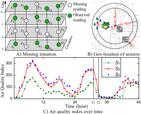
2) Affected by multiple complex factors, sensor readings change over location and time significantly and non-linearly. First, the readings of sensors with a shorter distance may not always be more similar than those with a farther distance. As illustrated in Figure 1 B), 𝑠1 is closer to 𝑠2 than 𝑠3 in terms of geographical Euclidian Distance. As shown in Figure 1 C), however, the air quality readings of 𝑠2 are more similar to 𝑠3
than 𝑠1. The reason is that 𝑠2 and 𝑠3 are located in two regions with a similar geographical context, such as Point of Interests and traffic patterns, while 𝑠1 is deployed in a forest and with a lake between it and 𝑠2. These cases violate the First Law of Geography, devaluing some interpolation-based models, like Inverse Distance Weighting (IDW) [George and Wong, 2008]. Second, sensor readings fluctuate tremendously over time, sometimes coming with a sudden change. As illustrated in Figure 1 C), the reading of 𝑠2 at the 31st timestamp drops over 200 in two hours. Such sudden change is actually very important to real-time monitoring and further data analysis, but cannot be well handled by existing smoothing or interpolation methods.
To tackle these challenges, we propose a spatio-temporal multi-view-based learning (ST-MVL) method to collectively fill missing values in a set of geo-sensory readings from a spatio-temporal and global-local perspectives simultaneously. Our contributions are four-fold:
- x ST-MVL simultaneously considers 1) the spatial correlation between different time series and 2) the temporal correlation between readings at different timestamps in the same series, to generate a more accurate estimate.
- x ST-MVL integrates the advantages of global views, i.e. empirical models derived from the data over a long period, and those of local views, i.e. data-driven algorithms that are concerned with recent readings, to achieve better accuracy.
- x ST-MVL can handle the block missing problem, combining the four views in a multi-view learning framework.
- x We evaluate our method using Beijing air quality and meteorological data. The results demonstrate the advantages of our method compared with ten baselines.
2 Overview
Figure 2 presents 𝑚 sensors' readings at 𝑛 consecutive timesamps, which are stored in a form of matrix, where a row stands for a sensor and a column denotes a timestamp. An entry 𝑣𝑖𝑗 refers to the reading of 𝑖 𝑡ℎ sensor at 𝑗𝑡ℎ timestamp. In this matrix, 𝑣2𝑗 and 𝑣1,𝑗+1 are missing. We can estimate the reading of 𝑣2𝑗 based on its spatial neighborhoods, such as 𝑠1 and 𝑠3; we call it a spatial view. 𝑣2𝑗 can also be estimated based on readings of adjacent timestamps, like 𝑡𝑗-1 and 𝑡𝑗+1, etc.; we call it a temporal view. We can also use different time length of data for an estimation, enabling local and global views. For example, we consider adjacent readings of 𝑣2𝑗 from 𝑡𝑗-2 to 𝑡𝑗+2 in a local data matrix, which is regarded as a local view. We define the number of columns in a local data matrix as a window size 𝜔. Alternatively, we can take into account readings over a very long time period, e.g. from 𝑡1 to 𝑡𝑛, which is regarded as a global view. Local view captures instantaneous changes, whereas global view represents longterm patterns. If the values of an entire row or a column in a local data matrix are missing, we call it a block missing problem.
| Temporal | ω=5 | ||||||||||
|---|---|---|---|---|---|---|---|---|---|---|---|
| t1 | t2 | ...... | tj-2 | tj-1 | tj | tj+1 | tj+2 | ...... | tn-1 | tn | |
| s1 Spatial | 230 | 230 | . | 205 | 164 | 185 | 188 | . | 223 | 249 | |
| s2 | 200 | 188 | . | 173 | 136 | 146 | 185 | . | 199 | 255 | |
| s3 | 118 | 93 | . | 72 | 56 | 59 | 44 | 78 | . | 99 | 111 |
| Local | |||||||||||
| sm | 121 | 102 | . | 60 | 30 | 40 | 33 | 56 | . | 88 | 106 |
Global
Figure 2: Data matrix of sensor readings
As shown in Figure 3, ST-MVL consists of four views: IDW, Simple Exponential Smoothing (SES), User-based Collaborative filtering (UCF) and Item-based Collaborative filtering (ICF). The four views are then aggregated to generate a final estimate for a missing reading.
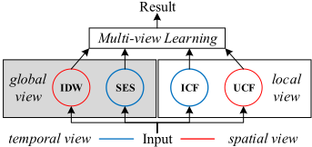
IDW computes an estimate for a missing reading of a sensor based on the readings of the sensor's spatial neighborhoods. SES estimates the missing reading of a sensor based on readings at other timestamps of the same sensor. As IDW and SES are actually empirical models derived from data over a long period of history, they denote a global spatial view and global temporal view on the missing reading respectively.
On the contrary, UCF estimates a missing reading only based on the local similarity between a sensor's recent readings and those of the sensor's spatial neighbors, where a sensor is regarded as a user. Likewise, ICF estimates a missing reading based on the local similarity between recent readings of different timestamps, where a timestamp denotes an item. As UCF and ICF only consider local similarity from a spatial and temporal perspective, they stand for local spatial and local temporal views respectively.
To leverage advantages of different views, we propose a multi-veiw learning algorithm that finds a linear combination of different views' predictions with minimal square errors.
3 The ST-MLV Method
In this section, we detail ST-MLV, using a running example to fill the reading of 𝑣2𝑗 shown in Figure 2. In the following, the term "missing value" equals "missing reading".
3.1 Global Spatial View - IDW
To model the global spatial view, we employ a statistic model, IDW, to interpolate a missing value based on its spatial neighborhoods. IDW assigns a weight to each available reading of geospatially adjacent sensors according to their distance to the target sensor, and aggregates these weights by Equation (1) to make prediction 𝑣̂𝑔𝑠.
where 𝑑𝑖 is the spatial distance between a candidate sensor 𝑠𝑖 and the target sensor, and α is a positive power parameter that controls the decay rate of a sensor's weight by 𝑑𝑖 -𝛼 . 𝑑𝑖 -𝛼 assigns a bigger weight to closer sensors' readings, for which a bigger 𝛼 denotes a faster decay of weight by distance.
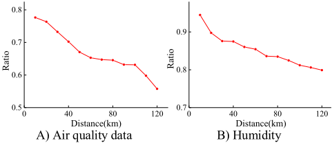
Figure 4 presents the statistics that motivate us to use IDW to model global spatial view, using two datasets: air quality data and meteorological data in Beijing from May 2014 to May 2015. Here, we calculate the ratio between arbitrary two sensors' readings at the same timestamp. The ratio decreases as the distance between two sensors increases in both datasets. This actually follows the First Law of Geography [Tobler, 1970], i.e. Everything is related to everything else, but near things are more related than distant things, which is an empirical spatial correlation in geo-sensory data.
Here, we demonstrate IDW using the running example. Suppose two sensors 𝑠1 and 𝑠3 are near 𝑠2 with spatial distance 6.5km and 8.5km respectively. If setting 𝛼 = 1, weights to two sensors are 1/6.5 and 1/8.5. Then, we get the prediction 𝑣̂𝑔𝑠=130 after weighting average.
3.2 Global Temporal View - SES
To incorporate the global temporal view, we utilize SES to estimate the missing value based on the readings of same sensor at other timestamps. SES is frequently used in the time series domain as an exponential moving average model, formally defined as [Gardner, 2006]:
where 𝑡𝑗 is a time interval between a candidate reading 𝑣𝑗 and a target reading; 𝛽 is a smoothing parameter with a range of (0, 1). In general, 𝛽 ∗ (1 -𝛽)𝑡-1 gives a bigger weight to recent readings than distance ones, and a smaller 𝛽 denotes a slower decay of weight over the time interval. Traditional SES uses only predecessors of the target timestamp as input. Here, we extend it to use both predecessors and successors of a target timestamp. Given a target timestamp, our SES gives a weight 𝛽 ∗ (1 -𝛽)𝑡-1 to each reading of the same sensor, calculating 𝑣̂𝑔𝑡 by normalizing the weight according to Equation (3):
In implementation, we only select readings within a temporal threshold (12 hours), as distant reading is not very useful.
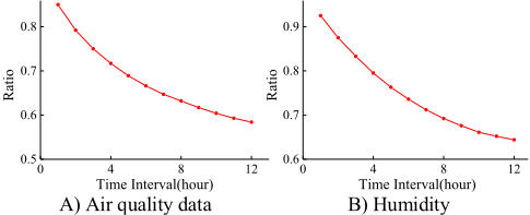
Our SES model is inspired by the observation from time series data. Figure 5 presents the ratio between arbitrary two readings at two different timestamps of the same sensor, using the same air quality data an meteorological data presented in Figure 4. Both curves in Figure 5 decrease as the time interval increases, showing an empirical temporal correlation in time series, i.e. readings of recent timestamps are more relevant than readings of distant timestamps.
Following the running example, suppose we find four timestamps (𝑡𝑗-2, 𝑡𝑗-1, 𝑡𝑗+1, 𝑡𝑗+2) for 𝑡𝑗. If setting β = 0.5, the weights for the four timestamps are (0.25, 0.5, 0.5, 0.25) respectively. Thus, the final result 𝑣̂𝑔𝑡 equals to 185.
3.3 Local Spatial View - UCF
UCF is a data-driven algorithm that has been wildly used in recommender systems. The general idea behind it is similar users make similar ratings for similar items [Su and Khoshgoftaar, 2009]. Following the running example shown in Figure 2, we regard a sensor as a user, constructing a local data matrix for 𝑣2𝑗 with adjacent readings [𝑣∗(𝑗-𝜔-1 2 ) …𝑣∗(𝑗+𝜔-1 2 ) ], where 𝜔 is the windows size. The similarity between two sensors (𝑠𝑖 , 𝑠2) is measured based on readings in the local data matrix, according to Equation (4):
where 𝑁𝑇 is the number of timestamps that two sensors both have readings. We then calculate a weighted average 𝑣̂𝑙𝑠 using the similarity as a weight, according to Equation 5.
UCF deals with special cases where the empirical spatial correlation mentioned in Section 3.1 does not hold, e.g. the case shown in Figure 1 B), capturing the time-dependent (i.e. local) spatial correlation between sensors' readings.
3.4 Local Temporal View - ICF
Regarding a timestamp as a item, ICF [Sarwar et al., 2001] calculates the similarity between two timestamps (𝑡1, 𝑡2) based on recent readings in the local data matrix built in the UCF model, according to Equation (6):
where 𝑁𝑆 is the number of sensors that have readings in both 𝑡1 and 𝑡2 . We use the similarity as a weight to calculate weighted average 𝑣̂𝑙𝑡 with the readings [ 𝑣𝑗1 …𝑣𝑗2 ] whose timestamp is within window size 𝜔 of the local data matrix, according to Equation (7).
ICF, as local temporal view, deals with special cases where the empirical temporal correlation mentioned in Section 3.2 does not hold, using the time-dependent (i.e. local) temporal correlation learned from recent data.
3.5 Multi-View Learning
ST-MVL integrates the predictions of the aforementioned four views to generate a final result, through a multi-view learning algorithm, according to Equation (8):
where 𝑏 is a residual and 𝑤𝑖 ( 𝑖 =1,2,3,4) is a weight assigned to each view. Algorithm 1 presents the procedure of ST-MVL. When a dataset encounters a block missing problem, in which ICF and UCF do not work very well, we leverage IDW and SES to generate an initial value for those missing entries (see Line 3). Then, we predict each missing entry using ICF, UCF, IDW and SES respectively (Line 4-9), combining the four predictions based on a linear-kernelbased multi-view learning framework (see Line 10 and Equation 8). We train the model for each sensor respectively, by minimizing the linear least square error [Lawson and Hanson, 1974] between predictions and ground truth.
Algorithm 1 ST-MVL
Input: Original Data Matrix 𝑀, 𝜔, 𝛼, 𝛽; Output: Final Data Matrix; 1. O ← Get_All_Missing_Values(𝑀); 2. If there are block missing problem 3. 𝑀 ← Initialization(𝑀, 𝛼, 𝛽); 4. Foreach target t in O 5. 𝑣̂𝑙𝑠 ← UCF(𝑀, 𝑡,𝜔); 6. 𝑣̂𝑙𝑡 ← ICF(𝑀, 𝑡, 𝜔); 7. 𝑣̂𝑔𝑠 ← IDW(𝑀, 𝑡, 𝛼); 8. 𝑣̂𝑔𝑡 ← SES(𝑀, 𝑡, 𝛽); 9. 𝑣̂𝑚𝑣𝑙 ← Muti-view_Learning(𝑣̂𝑙𝑠, 𝑣̂𝑙𝑡, 𝑣̂gs, 𝑣̂𝑔𝑡); 10. Add 𝑣̂𝑚𝑣𝑙 into 𝑀;//using IDW or SES 11. Return 𝑀;4 Experiments
4.1 Datasets and Ground Truth
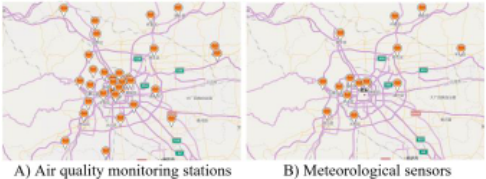
We evaluate our model based on two real datasets: air quality and meteorological data in Beijing from 2014/05/01 to 2015/04/30 [Zheng et al., 2015], which has 8,759 timestamps respectively. The air quality data is collected at 36 air quality monitoring stations, each of which generates a reading every hour, as depicted in Figure 6 A). The meteorological data is collected by 16 sensors shown in Figure 6 B) every hour.
From the two datasets, we select 4 properties, consisting of PM2.5, NO2, Humidity and WindSpeed, to fill missing values whose statistics are shown in Table 1. There are two missing situations: block missing and general missing. The former is further comprised of spatial block missing and temporal block missing; the two may have some overlap. The spatial block missing is referred to as records with all sensors' readings simultaneously absent; the temporal block missing is records of the same sensor with data absent in a certain temporal window size (see Figure 2, e.g. there are 3.15% of missing values in PM2.5 property when ω = 11). General missing is the missing values except for the block missing. For example, about 13.25% of sensor readings in the air quality dataset lose PM2.5 property, including 8.15% general missing and 2.15% spatial block missing.
| PM2.5 | NO2 | Humid ity | Wind Speed | ||
|---|---|---|---|---|---|
| Block | Spatial | 2.2% | 3.9% | 9.8% | 11.8% |
| missing | Temporal (ω=11) | 3.5% | 6.5% | 9.6% | 19.5% |
| General missing | 8.2% | 6.8% | 4.6% | 4.0% | |
| Overall | 13.3% | 16.0% | 21.5% | 30.3% | |
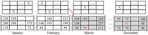
We partition the 1-year data into two parts, using the 3rd, 6th, 9th and 12th months as a test set and the rest for a training set. To train our model, we select entries (from the training set) whose local matrix is not totally absent of data at the row and column where the entry stays. As illustrated in Figure 7, for the test set, we accommodate each month's data into a matrix respectively. We find all missing entries (denoted by red X) in each month's data. Then, we drop out the values of entries (in the next month's matrix e.g. 𝑣32 in March) that correspond to its predecessor's (i.e. Feb.) missing entries. If those entries are not absent in the next month (e.g. 𝑣32=59 in March), their values are used as a ground truth to measure the accuracy of our predictions. Note that we cannot randomly drop out some non-missing entries in the test set to generate ground truth, as real-world missing patterns are not random.
4.2 Baselines & Metrics & Prameters
We compare our method with 10 baselines shown in Table 2. ARMA& SARIMA: ARMA predicts a missing value based on the readings of a few timestamps ago. SARIMA generalizes ARMA, considering the seasonal factor in time series. stKNN: This uses the average readings of its k nearest spatial and temporal neighbors as a prediction (𝑘=6).
Kriging: Kriging interpolates a missing value with available readings of geospatially adjacent sensors.
AKE (Applying k-nearest neighbor estimation) [Pan and Li, 2010]: It uses a regression model to combine the readings of a missing entry's neighbors.
DESM: Combines previous readings of a missing sensor and its neighbors' readings at current time linearly, using statistic based spatio-temporal correlations. [Gruenwald et al., 2010]. IDW+SES: Fill missing entries in a sensor's local matrix by IDW and SES respectively; return the average of predictions. CF: Initialize a local matrix by IDW+SES; apply UCF and ICF to generate a prediction respectively; the return is the average of the two predictions.
NMF: Initialize a local matrix by IDW+SES; fill the local matrix by a NMF.
NMF-MVL: Similar to our method, but it replaces two local views with a NMF.
| Method | Spatial | Temporal | Spatial+Temporal |
|---|---|---|---|
| Global | IDW | SES | IDW+SES |
| Lobal | UCF | ICF, ARMA | CF, NMF, stKNN |
| Global+Local | Kriging | SARIMA | AKE, DESM, NMF-MVL |
Evaluation Metrics: We measure our mehtod by Mean Absolute Error (MAE) and Mean Relative Error (MRE),
where 𝑣𝑖 ̂ is a prediction and 𝑣𝑖 is the ground truth; 𝑛 is the number of cases.
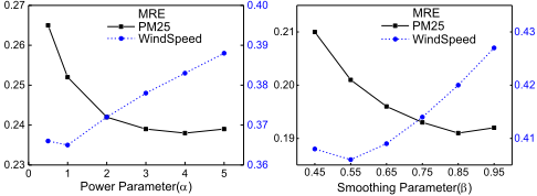
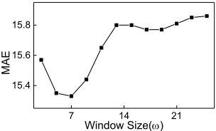
Parameter Settings: We test different 𝛼 for IDW, 𝛽 for SES, and 𝜔 for UCF & ICF, finding a best setting for them, e.g. when 𝛼=4, 𝛽=0.85, and 𝜔=7 achieve the best performance in PM2.5 property.
4.3 Results
4.3.1 Results of Combination Methods
Table 3 presents the results of different combination methods of four views, based on PM2.5 property. ST-MVL outperforms all kinds of combinations, bringing a significant improvement beyond the best single view SES and the best combination of two views (IDW+SES). ST-MVL also achieves a slightly better performance in filling in block missing than others. In the meantime, the combination of two views, e.g. IDW+SES, is better than using a single view; same for UCF+ICF. The four views are complementary to each other, containing long-term patterns, knowledge derived from recent contexts, the spatial correlation between locations, and the temporal correlation between timestamps. Additionally, IDW and SES have better results than UCF and ICF respectively, showing the ability of empirical models dealing with general cases.
| Method | General Missing | Spatial Block Missing | Temporal Block Missing | |||
|---|---|---|---|---|---|---|
| MAE | MRE | MAE | MRE | MAE | MRE | |
| IDW | 15.20 | 0.222 | \ | \ | 11.95 | 0.213 |
| Global SES | 13.39 | 0.196 | 18.25 | 0.215 | \ | \ |
| IDW+SES | 11.64 | 0.171 | 18.25 | 0.215 | 11.95 | 0.213 |
| UCF | 13.49 | 0.206 | \ | \ | \ | \ |
| Lobal ICF | 15.37 | 0.234 | \ | \ | \ | \ |
| UCF+ICF | 11.73 | 0.178 | \ | \ | \ | \ |
| Spa:IDW+UCF | 16.14 | 0.235 | \ | \ | 11.95 | 0.213 |
| Tem:SES+ICF | 13.57 | 0.199 | 18.25 | 0.215 | \ | \ |
| ST-MVL | 10.81 | 0.158 | 17.85 | 0.217 | 11.71 | 0.208 |
Note: Spa means Spatial; tem means Temporal.
4.3.2 Overall Results
Table 4 presents the comparison between our method and ten baselines, where ST-MVL outperforms all baselines under all circumstances. Sudden changes denote the readings changing over the last timestamp by a threshold (e.g. 50 in our settings). We use IDW+SES to initialize the missing values for datadriven algorithms, such as CF and NMF, when the latter faces block missing. Individually, NMF outperforms CF, as it considers user and item similarities simultaneously. However, when combined with other views in the multiview learning framework, CF brings a bigger improvement over NMF, i.e. ST-MVL outperforms NMF-MVL.
| Method | General Missing | Spatial Block Missing | Temporal Block Missing | Sudden Change | Overall | |||||
|---|---|---|---|---|---|---|---|---|---|---|
| MAE | MRE | MAE | MRE | MAE | MRE | MAE | MRE | MAE | MRE | |
| ARMA | 22.61 | 0.331 | 29.26 | 0.369 | \ | \ | 51.11 | 0.567 | 27.47 | 0.394 |
| Kriging | 15.53 | 0.221 | \ | \ | 15.62 | 0.222 | 42.32 | 0.407 | 16.59 | 0.234 |
| SARIMA | 14.69 | 0.220 | 23.92 | 0.319 | 31.20 | 0.561 | 52.80 | 0.586 | 18.76 | 0.278 |
| stKNN | 12.84 | 0.188 | 19.91 | 0.235 | 12.72 | 0.226 | 35.13 | 0.390 | 14.00 | 0.201 |
| DESM | 13.65 | 0.191 | 19.24 | 0.233 | 12.66 | 0.224 | 42.87 | 0.425 | 15.59 | 0.228 |
| AKE | 13.34 | 0.195 | 19.08 | 0.229 | 12.14 | 0.22 | 41.54 | 0.403 | 14.27 | 0.211 |
| IDW+SES | 11.64 | 0.171 | 18.25 | 0.215 | 11.95 | 0.213 | 34.33 | 0.381 | 12.70 | 0.183 |
| CF | 12.20 | 0.178 | 19.27 | 0.234 | 12.25 | 0.218 | 34.91 | 0.388 | 13.40 | 0.193 |
| NMF | 11.21 | 0.163 | 18.98 | 0.239 | 12.73 | 0.217 | 34.37 | 0.381 | 13.08 | 0.188 |
| NMF-MVL | 11.16 | 0.162 | 18.97 | 0.238 | 12.66 | 0.217 | 34.33 | 0.380 | 13.06 | 0.187 |
| ST-MVL | 10.81 | 0.158 | 17.85 | 0.217 | 11.71 | 0.208 | 33.15 | 0.368 | 12.12 | 0.174 |
4.3.3 Impact of Parameters for IDW & SES
Figure 8 A) plots the performance of IDW changing over 𝛼 in PM2.5 and WindSpeed datasets. PM2.5 has a minimum MRE when 𝛼=4, and WindSpeed has a minimum MRE when 𝛼=1. Figure 8 B) shows the performance of SES changing over 𝛽. When 𝛽=0.85 and 0.55, PM2.5 and WindSpeed have a minimum MRE respectively. As PM2.5 fluctuates more strongly than wind speed in both spatial and temporal spaces, the latter should be given a smaller 𝛼 and 𝛽.
4.3.4 Impact of Window Size for CF
Figure 9 shows the impact of window size on CF. A large window size may lose time-dependency, but a very small window size may not capture the similarity between locations or time stamps. That is why MAE decreases first and then increases after 𝜔=7.
4.3.5 Results in Other Datasets
Table 5 presents the results of all properties of the two datasets. ST-MVL outperforms IDW+SES in all properties, achieving an improvement of 0.009 in MRE with the multi-view learning. It verifies the advantages of our method integrating empirical models and data-driven algorithms.
| Dataset | IDW+SES | ST-MVL | ||
|---|---|---|---|---|
| MAE | MRE | MAE | MRE | |
| PM2.5 | 12.70 | 0.183 | 12.12 | 0.174 |
| NO2 | 8.93 | 0.176 | 8.45 | 0.171 |
| WindSpeed | 2.91 | 0.427 | 2.74 | 0.411 |
| Humidity | 4.14 | 0.085 | 3.82 | 0.079 |
5 Related Work
5.1 Methods Considering a Single View
Spatial models: Inverse distance weighting, linear regression and Kriging are three wildly used methods. [Chen and Liu, 2012] estimates the rainfall distribution using inverse distance weighting, and [Wu and Li, 2013] fills the missing temperature using ordinary Kriging. These methods leverage the spatial correlation derived from the spatial coordinates data or learnt from data.
Temporal models: Methods in this category can be classified into non-feature-based and feature-based. The former, such as SES, ARMA and SARIMA, solely considers a sensor's readings [Ceylan et al., 2013]. The latter, such as Graph model and regression model [Lee et al., 2008; Fung, 2006], exploits a function of features, considering the temporal correlation of readings over time.
Beyond the aforementioned two categories of methods solely considering spatial information or temporal information, our method simultaneously utilizes spatial and temporal correlations, and therefore is more capable of filling in missing values.
5.2 Methods Considering Spatio-Temporal Views
Many statistic-based methods, such as mean imputation and last seen [Little and Rubin, 2014], can be used to impute the missing data. In addition, there are many data-driven methods for filling missing values. [Gruenwald et al., 2010] proposes a DEMS method to handle the missing data by time-dependent spatial and temporal relationships. [Pan and Li, 2010] proposes a nearest neighbors imputation method entitled AKE to describe the spatial correlation and incorporate the temporal information when meeting no enough spatial information. [Wang et at., 2006; Ma et al., 2007] unify user-based and item-based collaborative filtering to fill missing values in the recommendation system. [Johan at el., 2014] takes advantage of matrix factorization and a salient version called empirical orthogonal functions model is proposed by [Antti et al., 2010]. In general, statistic-based methods are derived from history data, characterizing the global information; Data-driven methods focus on the recent contexts, characterizing the local information. Our method combines the statistic models and data-driven models in a multi-view learning framework to generate a more accurate estimate.
6 Conclusion
In this paper, we propose a multi-view learning-based method to fill missing values for geo-sensory time series data, simultanesouly considering spatial, temporal, global and local views. We evaluate our method ST-MVL based on Beijing's air quality and meteorological data. ST-MVL has a mean relative error around 17% for PM2.5 and NO2, and about 8% for humidity, outperforming baseline methods that solely consider a single view by 26% on average. ST-MVL also surpasses those that only combine two out of the four views by 10% in MRE on average. The code and datasets have been released at: http://research.microsoft.com/apps/pubs/?id=264768.
Acknowledgments
This work was supported by the China National Basic Research Program (973 Program, No. 2015CB352400) and the National Natural Science Foundation of China (Nos. U1401258, 61573292).
@inproceedings{ijcai2016p384,
  title     = {ST-MVL: Filling Missing Values in Geo-Sensory Time Series Data},
  author    = {Yi, Xiuwen and Zheng, Yu and Zhang, Junbo and Li, Tianrui},
  booktitle = {Proceedings of the Twenty-Fifth International Joint Conference on
               Artificial Intelligence, {IJCAI-16}},
  publisher = {AAAI Press / International Joint Conferences on Artificial Intelligence},
  editor    = {Subbarao Kambhampati},
  pages     = {2704--2709},
  year      = {2016},
  month     = {7},
  url       = {https://ijcai.org/proceedings/2016/384},
}
TY - CPAPER TI - ST-MVL: Filling Missing Values in Geo-Sensory Time Series Data AU - Yi, Xiuwen AU - Zheng, Yu AU - Zhang, Junbo AU - Li, Tianrui T2 - Proceedings of the Twenty-Fifth International Joint Conference on Artificial Intelligence, IJCAI-16 PB - AAAI Press / International Joint Conferences on Artificial Intelligence PY - 2016 SP - 2704 EP - 2709 UR - https://ijcai.org/proceedings/2016/384 ER -Copied
Machine-readable versions of this paper, for tools and AI agents:





