
Situation Testing-Based Discrimination Discovery: A Causal Inference Approach
Proceedings of the Twenty-Fifth International Joint Conference on Artificial Intelligence. Pages 2718-2723.
Abstract
Discrimination discovery is to unveil discrimination against a specific individual by analyzing the historical dataset. In this paper, we develop a general technique to capture discrimination based on the legally grounded situation testing methodology. For any individual, we find pairs of tuples from the dataset with similar characteristics apart from belonging or not to the protected-by-law group and assign them in two groups. The individual is considered as discriminated if significant difference is observed between the decisions from the two groups. To find similar tuples, we make use of the Causal Bayesian Networks and the associated causal inference as a guideline. The causal structure of the dataset and the causal effect of each attribute on the decision are used to facilitate the similarity measurement. Through empirical assessments on a real dataset, our approach shows good efficacy both in accuracy and efficiency.
- [Bendick, 2007] Marc Bendick. Situation testing for em- ployment discrimination in the united states of america. Horizons stratégiques, (3):17-39, 2007.
- [Bonchi et al., 2015] Francesco Bonchi, Sara Hajian, Bud Mishra, and Daniele Ramazzotti. Exposing the proba- bilistic causal structure of discrimination. arXiv preprint arXiv:1510.00552, 2015.
- [Calders and Verwer, 2010] Toon Calders and Sicco Ver- wer. Three naive bayes approaches for discrimination-free classification. Data Mining and Knowledge Discovery, 21(2):277-292, 2010.
- [Colombo and Maathuis, 2014] Diego Colombo and Mar- loes H Maathuis. Order-independent constraint-based causal structure learning. The Journal of Machine Learn- ing Research, 15(1):3741-3782, 2014.
- [Foster, 2004] Sheila R Foster. Causation in antidiscrimi- nation law: Beyond intent versus impact. Hous. L. Rev., 41:1469, 2004.
- [Glymour and others, 2004] Clark Glymour et al. The TETRAD project. http://www.phil.cmu.edu/tetrad, 2004. Link
- [Hajian and Domingo-Ferrer, 2013] Sara Hajian and Josep Domingo-Ferrer. A methodology for direct and indirect discrimination prevention in data mining. Knowledge and Data Engineering, IEEE Transactions on, 25(7):1445- 1459, 2013.
- [Hajian et al., 2015] Sara Hajian, Josep Domingo-Ferrer, Anna Monreale, Dino Pedreschi, and Fosca Giannotti. Discrimination-and privacy-aware patterns. Data Mining and Knowledge Discovery, 29(6):1733-1782, 2015.
- [Kamiran and Calders, 2009] Faisal Kamiran and Toon Calders. Classifying without discriminating. In 2nd International Conference on Computer, Control and Communication (IC4 2009), pages 1-6. IEEE, 2009.
- [Kamiran and Calders, 2012] Faisal Kamiran and Toon Calders. Data preprocessing techniques for classification without discrimination. Knowledge and Information Systems, 33(1):1-33, 2012.
- [Kamishima et al., 2011] Toshihiro Kamishima, Shotaro Akaho, and Jun Sakuma. Fairness-aware learning through regularization approach. In Data Mining Workshops (ICDMW), 2011 IEEE 11th International Conference on, pages 643-650. IEEE, 2011.
- [Koller and Friedman, 2009] Daphne Koller and Nir Fried- man. Probabilistic graphical models: principles and tech- niques. MIT press, 2009.
- [Luong et al., 2011] Binh Thanh Luong, Salvatore Ruggieri, and Franco Turini. k-nn as an implementation of situa- tion testing for discrimination discovery and prevention. In Proceedings of the 17th ACM SIGKDD international con- ference on Knowledge discovery and data mining, pages 502-510. ACM, 2011.
- [Mancuhan and Clifton, 2014] Koray Mancuhan and Chris Clifton. Combating discrimination using bayesian net- works. Artificial intelligence and law, 22(2):211-238, 2014.
- [Neapolitan and others, 2004] Richard E Neapolitan et al. Learning bayesian networks, volume 38. Prentice Hall Upper Saddle River, 2004. [Netherlands, 2001] Statistics Netherlands. Volkstelling. https://sites.google.com/site/faisalkamiran/, 2001. Link
- [Pearl, 2001] Judea Pearl. Direct and indirect e↵ects. In Pro- ceedings of the seventeenth conference on uncertainty in artificial intelligence, pages 411-420.
- Morgan Kaufmann Publishers Inc., 2001. [Pearl, 2009] Judea Pearl. Causality. Cambridge university press, 2009.
- [Pedreschi et al., 2009] Dino Pedreschi, Salvatore Ruggieri, and Franco Turini. Measuring discrimination in socially- sensitive decision records. In Society for Industrial and Applied Mathematics. Proceedings of the SIAM Interna- tional Conference on Data Mining, page 581. Society for Industrial and Applied Mathematics, 2009.
- [Pedreshi et al., 2008] Dino Pedreshi, Salvatore Ruggieri, and Franco Turini. Discrimination-aware data mining. In Proceedings of the 14th ACM SIGKDD international con- ference on Knowledge discovery and data mining, pages 560-568. ACM, 2008.
- [Romei and Ruggieri, 2014] Andrea Romei and Salvatore Ruggieri. A multidisciplinary survey on discrimina- tion analysis. The Knowledge Engineering Review, 29(05):582-638, 2014.
- [Rorive, 2009] Isabelle Rorive. Proving discrimination cases: The role of situation testing. 2009.
- [Ruggieri et al., 2010] Salvatore Ruggieri, Dino Pedreschi, and Franco Turini. Data mining for discrimination dis- covery. ACM Transactions on Knowledge Discovery from Data (TKDD), 4(2):9, 2010.
- [Spirtes et al., 2000] Peter Spirtes, Clark N Glymour, and Richard Scheines. Causation, prediction, and search, vol- ume 81. MIT press, 2000.
- [Wu and Wu, 2015] Yongkai Wu and Xintao Wu. Using log- linear model for discrimination discovery and prevention. Technical Report DPL-2015-002, University of Arkansas, 2015.
- [Zhang et al., 2016] Lu Zhang, Yongkai Wu, and Xintao Wu. Situation testing-based discrimination discovery: A causal inference approach. Technical Report DPL-2016-002, University of Arkansas, 2016.
- [Zliobaite et al., 2011] Indre Zliobaite, Faisal Kamiran, and Toon Calders. Handling conditional discrimination. In Data Mining (ICDM), 2011 IEEE 11th International Con- ference on, pages 992-1001. IEEE, 2011.
References were extracted automatically from the PDF and may contain errors.
Full text extracted automatically from the PDF; figures, tables and equations may differ. The PDF is the version of record.
1 Introduction
Discrimination refers to the unjustified distinction against an individual based on the group, class or category to which that individual belongs or is perceived to belong. Discrimination is widespread in subjective decision making processes. This situation even deteriorates today due to the increased use of predictive models that are built around the collection of individual data to make important decisions like employment, credit, insurance, etc. A large number of laws and regulations (e.g., Council Directive 2000/78/EC or Title VII of the Civil Rights Act of 1964) have been established to forbid discrimination on several grounds, such as gender, age, pregnancy, sex orientation, race, national origin, religion, genetic information, and disability or illness, which are referred to as the protected attributes. Although the laws and regulations for discrimination are clear, proving discrimination in practice is difficult, because discrimination is usually hidden behind various pretexts and it is hard to find clear and sufficient evidence of discrimination in many cases [Rorive, 2009].
Discrimination discovery has been an active research area in data mining recently [Hajian and Domingo-Ferrer, 2013; Kamiran and Calders, 2012; Ruggieri et al., 2010; Romei and Ruggieri, 2014]. To detect discrimination against specific individuals, some researchers proposed to simulate situation testing using data mining algorithms over a historical decision dataset [Luong et al., 2011]. Situation testing is a legally grounded technique for analyzing the discriminatory treatment on an individual. It has been widely adopted both in the United States [Bendick, 2007] and the European Union [Rorive, 2009]. Situation testing is carried out in responding to a complaint about discrimination from an individual. Pairs of testers who are similar to the individual are then sent out to participate in the same decision process (e.g., applying for the same job). For each pair, the two testers possess the same characteristics except the membership to the protected group. For example, in the case of employment, the resumes of a pair of testers with di↵erent gender can be made equivalent in the education background, work experience, expertise and skills, and only vary in details and formats to avoid being considered as duplicates. The objective is to measure the treatments or decisions given to the members from the same pair. If one of the pair receives a di↵erent decision, the distinction implies discriminatory behavior. To ensure representativeness and "average out" random circumstances, a certain number of tester pairs are usually required by the court.
Employing the situation testing methodology, discrimination can be detected by finding a representative group of tuples from the historical dataset for a target individual. The representative group contains pairs of tuples with similar characteristics apart from belonging to the protected group and non-protected group. The target individual is considered as discriminated if significant di↵erence is observed between the decisions from the two parts of tuples. The key issue in the implementation of situation testing is how to define and determine the representative group. Luong et al. proposed a K-nearest neighbor (K-NN) classification based approach to find the similar tuples [Luong et al., 2011]. In their method, the similarity between two tuples is modeled via a distance function that takes all attributes as the input. The normalized Manhattan distance and overlap measurement are adopted to compute the distance between two tuples. Their approach shows a successful implementation of the situation testing methodology, however, there are several limitations: 1) They use all attributes for computing the distance. However, not all attributes are relevant to the decision, even if they are legally admissible. 2) The distance function does not distinguish the potentially di↵erent e↵ects on discrimination due to di↵erent values taken by an attribute. As a result, the identified representative group may not be accurate and the following situation testing could have incorrect results, as demonstrated in our empirical evaluations.
| No. | gender | major | score | height | weight | admission |
|---|---|---|---|---|---|---|
| 1 | F | CS | B | low | low | reject |
| 2 | M | CS | B | high | high | admit |
| 3 | F | CS | A | low | low | reject |
| 4 | M | CS | A | median | median | admit |
| 5 | F | CS | C | low | median | reject |
| 6 | M | CS | C | high | median | reject |
| 7 | M | EE | B | low | low | reject |
| ...... |
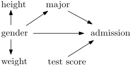
We propose the use of the Causal Bayesian Networks (CBNs) as a guideline in the implementation of situation testing for discrimination discovery. A CBN is a probabilistic graph model which is widely used for causality representation, reasoning and inference [Pearl, 2009]. Our ideas are as follows. First, only the attributes that are the direct causes of the decision should be used in the distance computation. Second, the causal e↵ect of an attribute on the decision can be used to facilitate the measurement of distance between di↵erent values taken by the attribute. Consider a toy model for a university admission system shown in Figure 1 and Table 1, which we use as the illustrative example throughout the paper. Intuitively, height and weight should not be involved in the distance computation as they are irrelevant to the decision. On the other hand, suppose that score grades A, B, C stand for good, median, and failure. It would be more reasonable if the A-to-B distance is measured smaller than the B-to-C distance.
In this paper, we develop a situation testing-based technique to capture discrimination with the support of the CBN. To find similar tuples, we define a distance function on the set of attributes that are the direct causes of the decision. For each attribute, we measure the distance between two domain values taking into consideration the value di↵erence as well as the causal e↵ect on the decision of changing the attribute from one value to the other. Through empirical assessments on a real dataset, we show that both the identification accuracy and efficiency can be significantly improved.
2 Preliminary Concepts
2.1 Data Representation
We consider a historical dataset that consists of a set T of tuples, each of which describes the profile of an individual.
Each tuple t 2 T is explicitly specified by a set of attributes, which contains some protected attributes, the decision attribute, and the non-protected attributes. In the illustrative example, gender is the protected attribute, admission is the decision attribute, and all the other attributes are the nonprotected attributes. Throughout this paper, we use an uppercase alphabet, e.g., X, to represent an attribute, e.g., major; a bold uppercase alphabet, e.g., X, to represent a subset of attributes, e.g., {major, score}. We use a lowercase alphabet, e.g., x, to represent a domain value of attribute X; a bold lowercase alphabet, e.g., x, to represent a value assignment of X. For ease of representation, we assume that there is only one protected attribute. We denote the protected attribute by C, associated with domain values of the protected group c - (e.g., female) and the non-protected group c + (e.g., male); and denote the decision by E, associated with domain values of positive decision e + and negative decision e - . The set of all the other non-protected attributes is denoted by R. Thus, a tuple t can be specified by the triple (c, r, e). Our approach can extend to handle multiple domain values of C/E and even multiple Cs.
2.2 Causal Bayesian Network
A CBN is a probabilistic graph model which is specified by a directed acyclic graph (DAG) G = (V,A) and a group of conditional probability distributions. V is a set of nodes and A is a set of arcs. In the DAG, each node represents an attribute. Each arc, denoted by an arrow ! pointing from the cause to the e↵ect, represents the direct causality between the two attributes. The absence of an arc between two nodes represents a claim of zero direct e↵ect between the two attributes in all distributions. In this paper, we assume that arc C ! E is present in the CBN. This indicates that there exits some kind of causal e↵ect of C on E in the whole dataset. However, whether a tuple is discriminated or not cannot be identified via the presence of arc C ! E. The CBN satisfies the Markov assumption, i.e., each node X is independent of all its non-descendants conditional on its parents Par(X). We also use Par(X) to represent a value assignment of the parents of X if no unambiguity occurs in the context. Each node is associated with a conditional probability distribution, i.e., P(X|Par(X)). The joint probability distribution over all attributes can be computed using the factorization formula [Koller and Friedman, 2009].
The basis for causal inference in the CBN is to measure the impact of interventions. An intervention is an action that forces some subset X of attributes to take certain values x. The intervention is supposed to be e↵ective in the sense that the value assignment of X is completely determined by the intervention, and local in the sense that of all other attributes Y (Y = V\X) the conditional distributions P(Y|Par(Y)) are not a↵ected by the intervention. The CBN permits us to estimate post-intervention distributions from the pre-intervention distributions using the do-calculus [Pearl, 2009]. Formally, the intervention that sets the value of X to x is represented by do(X = x) or simply do(x). The post-intervention distribution on Y, i.e., P(y|do(x)), is readily expressed as a truncated factorization formula where P(y|Par(Y))|X=x means substituting any attributes in X involved in the conditional probability with the corresponding values in x. There is also a set of inference rules to facilitate the expression of the post-intervention distributions. For a DAG G and a subset of nodes X in G, let G X denote the graph obtained by deleting all arcs pointing to nodes in X, and let GX denote the graph obtained by deleting all arcs emerging from nodes in X. The following proposition [Pearl, 2009] states the inferences rules.
Proposition 1 (Rules of do-Calculus). Let G be the DAG of a CBN. For any disjoint subsets of nodes X, Y, Z, W, there are following rules.
- P(y|do(x), z,w) = P(y|do(x),w), if Y and Z are dseparated by X [ W in G X .
- P(y|do(x), do(z),w) = P(y|do(x), z,w), if Y and Z are d-separated by X [ W in G XZ .
- P(y|do(x), do(z),w) = P(y|do(x),w), if Y and Z are dseparated by X [W in G XZ 0 , where Z 0 is the nodes in Z that are not ancestors of any nodes in W in G X .
The above rules make use of the well-known d-separation criterion.
Definition 1 (d-Separation). A path p is said to be blocked by a set of nodes Z if and only if
- p contains a chain i ! j or a fork i m! j such that the middle node m is in Z, or
- p contains an collider i ! m j such that the middle node m is not in Z and no descendant of m is in Z.
A set Z is said to d-separate X from Y if and only if Z blocks all paths from X to Y.
3 Strength andWeakness of Modeling Discrimination as Direct Causal E↵ect
Typically, a discrimination claim means demonstrating a direct causal connection between protected attribute C and decision attribute E [Foster, 2004]. Thus, the CBN and the associated causal inference have an immediate application in discrimination analysis since the discriminatory e↵ect can be straightly represented by the direct causal e↵ect of C on E. Using Pearl's method [Pearl, 2001], we define the direct causal e↵ect as follows:
Definition 2. Given a tuple t = (c, r, e), the direct causal effect of protected attribute C on decision attribute E is defined as
where r is a value assignment of R and R is the set of all the other attributes.
Equation (2) indicates that discrimination can be identified by the response of the decision E to the change of the protected attribute C while fixing the values of all the other attributes R. Note that fixing r is di↵erent from conditioning on r. The simply use of P(e + |do(c + ), r)-P(e + |do(c - ), r) may create spurious associations between C and E even when there is no direct causal e↵ect of C on E.
To calculate Equation (2), we have the following lemma.
Lemma 1. Equation (2) is equivalent to
where q is the value assignment of Q and Q is E's parent set except C, i.e., Q = Par(E)\{C}.
The proof of this lemma is straightforward using Equation (1). Equation (3) implies that the response of E can be estimated from the dataset by the di↵erence in the decision of tuples with the same characteristics Q apart from belonging or not in the protected group.
However, there exists a practical limitation with the above measurement in situation testing. In litigation the courts usually require a certain number of tester pairs for situation testing to ensure representativeness [Rorive, 2009]. Researchers in situation testing suggest that there should be at least 50 tester pairs in a single testing [Bendick, 2007]. However, the tuples used for computing the probabilities in Equation (3) must come from the same subgroup specified by q. Thus, there is no guarantee that the number of these tuples can satisfy any given requirement.
Inspired by [Luong et al., 2011], we tackle this limitation by finding 2K tuples that are closest to the target tuple, where K can be designated by the court. The CBN can provide a guidance of finding tuples. Intuitively, we can first select the tuples from the subgroup specified by q, and then select the tuples from the following appropriate subgroups. The details of our method will be discussed in the next section.
4 Discrimination Discovery
In this section, we describe our causal inference approach for discrimination discovery. We formalize situation testing in our context. Given a target tuple t with c = c - and e = e - , we rank all the tuples according to their distances to t using a distance function defined on an appropriate subset of nonprotected attributes. Then, we select the tuples that are within top-2K highest in the ranking for one-to-one pairing. The selected tuples with c + are added into set S + , and the selected tuples with c - are added into set S - . We compare the proportion p1 of tuples with e + among the tuples in S + , and the proportion p2 of tuples with e + among the tuples in S - . The di↵erence between p1 and p2, i.e., p1 - p2 reflects the bias due to the membership to the protected group. If p1 - p2 is greater than a threshold ⌧, then t is considered as being discriminated. The value of threshold ⌧ used for discrimination depends on the law. For instance, the 1975 British legislation for sex discrimination sets ⌧ = 0.05, namely a 5% di↵erence.
We assume that we have a CBN that is compatible with the dataset. We also make a reasonable assumption that there is no arc pointing to C in the CBN, as the protected attribute is always an inherent nature of an individual. A CBN can be learned from data and expert knowledge. In the past decades, many algorithms have been proposed to learn CBNs, and they are proved to be quite successful [Spirtes et al., 2000; Neapolitan and others, 2004; Colombo and Maathuis, 2014].
How a CBN is constructed by a learning algorithm or domain experts and how to measure the quality of a CBN are beyond the scope of this paper.
In the following, we first present the distance function and then describe the discovery algorithm.
4.1 Distance Function
Consider two tuples t and t 0 , the distance function d(t, t 0 ) measures the dissimilarity between the two tuples. To define the distance function, researchers first establish a distance metric for measuring the per-attribute distance, and then compute the joint e↵ect by summing up all the per-attribute distances. In [Luong et al., 2011], the distance between two domain values rk and r 0 k of attribute Rk 2 R is defined as the value di↵erence, where the normalized Manhattan distance is employed for ordinal/interval attributes, and the overlap measurement is employed for categorical attributes. The normalized Manhattan distance is defined as:
where range is used to normalize the result, defined as the di↵erence between the maximum and the minimum of the attribute. The overlap measurement is defined as:
Overall, the di↵erence between t and t 0 is given by
where
As discussed in Section 1, the above distance function has two limitations. First, Equation (3) implies that the distance function should be defined on Q, since they are the direct causes of the decision. Other attributes are either not causally related to E or have the causal e↵ects on E that are transmitted by the direct causes. Including these attributes in the distance computation may lead to incorrect results in the similarity measurement. Consider the illustrative example in Section 1. Suppose that tuple 1 is the target for testing, and we want to find the closest tuple from the tuples listed in the table. If we use all non-protected attributes to compute the distance, tuples 3 and 7 are the closest ones as both of them have only one mismatch. However, from the CBN we can see that, height and weight are not causally related to admission and should not be involved in the computation. In fact, tuple 2 is closest to the target since their majors and scores are exactly the same.
Second, when measuring the per-attribute distance, the causal e↵ect of each attribute on the decision can reveal important information relating to similarity. The response of the decision to change of the attribute reflects the di↵erence in how the two domain values a↵ect the decision. Thus, two values can be considered to be closer if changing the attribute from one value to the other produces smaller influence on the decision. Consider the same above example and we want to measure the distance between di↵erence values of attribute score. The distance between A and B and the distance between B and C are measured as equivalent if only the value di↵erence is considered, e.g., using the Manhattan distance. However, from the tuples listed in the table we can see that, both the admission rates for A and B are 50%, and the admission rate for C is 0%. Thus, the causal e↵ect of score on decision can facilitate to more accurately characterize the similarity in situations where A and B are closer than B and C with respect to the admission. Furthermore, the perattribute distance should be instance dependent. For example, although both the score di↵erence between tuples 3 and 2 and that between tuples 3 and 7 are the same A-to-B di↵erence, they should not be equal since tuples 3 and 2 apply to the same major while tuple 7 applies to another.
Based on the first observation, we define the distance function on the basis of Q, where Q = Par(E)\{C}. For the second observation, we measure the causal e↵ect on the decision of each attribute Qk 2 Q. We model the change of Qk from qk to q 0 k as two interventions that force Qk to take that two values respectively while keeping all other attributes the same as q. According to the definition of interventions [Pearl, 2009], we define as follows:
Lemma 2. Given a tuple t, the response of the decision to the change of Qk from qk to q 0 k is given by
where P(e + |do(q)) is the e↵ect of the intervention that forces Q to take value q, and P(e + |do(q 0 k , q\{qk})) is the e↵ect of the intervention that forces Qk to take value q 0 k and other attributes in Q to take the same value as q.
Note that CE(qk, q 0 k ) is instance dependent. For di↵erent tuples, the measure would not be equal even for the same pair of qk, q 0 k if the tuples possess di↵erent profiles q. Then, we define the distance function for tuples t, t 0 as follows.
Definition 3. The distance between tuples t, t 0 is given by
In our distance function, the production of CE(qk, q 0 k ) and VD(qk, q 0 k ) can be interpreted in two aspects: (1) CE(qk, q 0 k ) can be considered as the weight of VD(qk, q 0 k ), indicating how significant this value di↵erence is with regard to the decision; (2) VD(qk, q 0 k ) can also be considered as the weight of CE(qk, q 0 k ), indicating to what extend this causal e↵ect is relating to the similarity between the two values. A more general version may include the scale parameters ↵, β for the two metrics CE and VD:
where Q = Par(E){C}.
In the following, we show how to calculate CE(qk, q 0 k ). Directly using Equation (1) involves summing over all values of the attributes in R [ {C}\Q, which is too tedious. Thus, we make use of the inference rules in Proposition 1. The result is given by the following lemma.
Lemma 3. Given a tuple t,
Proof. As defined in Equation (4), we have CE(qk, q 0 k ) = P(e + |do(q)) - P(e + |do(q 0 k , q\{qk})). By conditioning and summing over the values of C, we can write P(e + |do(q)) as
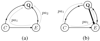
For term P(e + |c, do(q)), we can show that E and Q are dseparated given C in G CQ . Since all arcs pointing to C (in fact we have assumed that there is no arc pointing to C) and all arcs emerging from Q are deleted in G CQ , there are only two types of paths connecting E and Q, as illustrated in Figure 2a. The first type of paths pa1 starts from an arc pointing to E and ends with an arc pointing to any node in Q. Since C is the only parent of E in G CQ , pa1 must pass through C where C acts as the middle node in a fork. According to Condition 1 in Definition 1, pa1 is blocked by C. The second type of paths pa2 starts from an arc emerging from E and ends with an arc pointing to any node in Q. pa2 cannot consists entirely the arcs with the direction that points from E to Q, otherwise the mono-directional path E ! · · · Q ! E forms a circle in G, which contradicts to that G is a DAG. Thus, there exists at least one collider on pa2. According to Condition 2 in Definition 1, pa2 is blocked by ;. Therefore, E and Q are d-separated by C in G CQ . By applying Rule 2 in Proposition
1, we have
For term P(c|do(q)), as illustrated in Figure 2b, there is no arc pointing to C, and all arcs pointing to Q are deleted in G Q . Thus, there is only type of paths pa1, which starts with an arc emerging from C and ends with an arc emerging from any node in Q. Clearly, there must exist at least one collider on the path. According to Condition 2 in Definition 1, pa1 is blocked by ;. Therefore, C and Q are d-separated in G Q . By applying Rule 3 Proposition 1, we have
Thus, it follows that
Similarly we can calculate P(e + |do(q 0 k , q\{qk})). As a result, we have
⇤
4.2 Discovery Algorithm
Now we describe our discrimination discovery algorithm (CBN-DD). The pseudocode of the algorithm is presented in Algorithm 1. Given the target tuple t, the algorithm first finds the set Q in the CBN. Then, the algorithm is divided into three stages. In the first stage (lines 2-8), all tuples are ranked using the distance function (Equation (5)). Since the distance function is defined on Q, all the tuples are divided into homogeneous subgroups according to their value assignment of Q. All tuples in a subgroup are measured the same distance to t. Thus, the algorithm ranks the tuples on the basis of the subgroups. For each value assignment q l of Q, define subgroup g l = g l,+ [ g l,- containing all the tuples t 0 with q 0 = q l , where tuples with c 0 = c + are contained in g l,+ and tuples with c 0 = c - are contained in g l,- . Then, the distance d[l] is calculated between t and the first tuple in g l (denoted as g l [0]). The ranking orders are stored in an array L. In the second stage (lines 9-17), tuples that are ranked top-2K are selected, starting from subgroup g L[0] which ranks the highest. Within each subgroup g L[i] , we select the same number of tuples from g L[i],+ and g L[i],- to guarantee strict one-to-one pairing. The tuples selected from g L[i],+ are added into set S + , and tuples selected from g L[i],- are added into set S - . The algorithm selects as much as possible tuples from one subgroup, and then moves on to the next. The loop ends until the number of the selected tuples reaches 2K. Finally, in the third stage (lines 18-20), p1 and p2 are calculated from S + and S - , and the discrimination judgment is made based on p1 - p2.
The total computational complexity of the algorithm is O(M · |Q| + K), where M is the number of value assignments of Q. Usually, M is far smaller than the total number of tuples since Q is a subset of all the attributes.
5 Experiments
To evaluate the proposed discrimination discovery algorithm, we have conducted experiments by using the Dutch Census of 2001 [Netherlands, 2001], which is widely used in discrimination discovery literature. The dataset consists of 60421 tuples, each of which is described by 12 attributes. We treat sex (female and male) as the protected attribute and occupation (occupation w low income, occupation w high income) as the decision attribute. The CBN is constructed by TETRAD [Glymour and others, 2004], an open-source platform for causal modeling. We employ the original PC algorithm [Spirtes et al., 2000] and the significance level ↵ = 0.05 for the structure learning. For experiment details including the CBN please refer to our technical report [Zhang et al., 2016].
From the CBN, an arc from sex to occupation is observed, and the set Q is identified as {age, education level, country birth, economic status}. We randomly select 200 tuples as the targets for discrimination testing. For each target tuple, we search similar tuples
1 Q = Par(E)\{C}; 2 foreach value assignment q l of Q do 3 g l,+ = {t 0 |q 0 = q l , c 0 = c + }; 4 g l,- = {t 0 |q 0 = q l , c 0 = c - }; 5 g l = g l,+ [ g l,- ; 6 d[l] = d(t, g l [0]); 7 end 8 Rank g l in ascending order according to d[l] and store the orders in L[l]; 9 n = 0; i = 0; S + = S - = ;; 10 while n < K do 11 select min(|g L[i],+ |, |g L[i],- |, K - n) tuples t + from g l,+ ; 12 select min(|g L[i],+ |, |g L[i],- |, K - n) tuples t - from g l,- ; 13 S + = S + [ t + ; 14 S - = S - [ t - ; 15 n+ = |t + |; 16 i + +; 17 end 18 p1 = the positive decision rate in S + ; 19 p2 = the positive decision rate in S - ; 20 return p1 - p2 > ⌧ ? true : false;Table 2: Summarized results for 200 target tuples.
(a) Tuples identified as discriminated
(b) Accuracy
| K | CBN-DD | KNN-DD | ||||||
|---|---|---|---|---|---|---|---|---|
| K | CBN-DD | KNN-DD | di↵ | TP | TN | TP | TN | |
| 10 | 150 | 141.3 | 62.5 | 10 | 73.3 | 63.1 | 46 | 66.2 |
| 50 | 151.6 | 159.4 | 56 | 50 | 85.3 | 77.6 | 42.2 | 76.2 |
| 90 | 152.9 | 158.8 | 55.7 | 90 | 81.5 | 83.9 | 38.1 | 81.2 |
from the whole dataset. The threshold ⌧ is set as 0.05. We compare our algorithm (abbrev. as CBN-DD) with the algorithm in [Luong et al., 2011] (abbrev. as KNN-DD). We repeat the test 10 times. The average number of tuples identified as discriminated by the two algorithms as well as the number of di↵erent judgments for each tuple are shown in Table 2a. As can be seen, there is significant di↵erence between the judgments made by the two algorithms.
To measure the accuracy of the discrimination identification, we manually modify the dataset to obtain a data with ground truth. We first create a "clean" dataset by completely removing the attribute sex from the dataset and randomly assigning a gender to each tuple based on the original population. The "clean" dataset contains no bias against gender and hence each tuple can be labeled as "non-discriminated". Then, we manually introduce bias into the data. We simulate a situation where a domain user is responsible for making decisions and has a strong prejudice against females. So, he changes the decisions of 100 female tuples from positive to negative. We aim to evaluate how accurately two algorithms can identify them. For comparison, we also randomly select another 100 tuples that are labeled "non-discriminated" from the dataset and add them for testing. Similarly, the test is repeated 10 times and the average results of true positive (TP) and true negative (TN) are shown in Table 2b. It can be seen that, when K = 50, CBN-DD reports 85.3 tuples as discriminated among the 100 tuples that are true positive, and 77.6 tuples as non-discriminated among the 100 tuples that are true negative. In general, CBN-DD outperforms KNN-DD in both TP and TN for various values of K. For CBN-DD, TP decreases when K = 10 and K = 90. This is probably because of the randomness in selecting tuples when K is too small, and having to select dissimilar tuples when K is too large. How to suggest an appropriate K is left for future work.
The average CPU time for one target tuple is 0.3s for CBNDD and 20.3s for KNN-DD, showing that CBN-DD is much more computationally efficient than KNN-DD. Due to the large computational cost of KNN-DD, we only test 200 tuples in our evaluations.
6 RelatedWork
A number of data mining techniques have been proposed to discover discrimination in the literature. Pedreschi et al. proposed to extract from the dataset classification rules which represent certain discrimination patterns [Pedreshi et al., 2008; Pedreschi et al., 2009]. If the presence of the protective attribute increases the confidence of a classification rule, it indicates possible discrimination in the data set. Based on that, [Mancuhan and Clifton, 2014] further proposed to use the Bayesian network to compute the confidence of the classification rules for detecting discrimination. Di↵erently, conditional discrimination, where part of discrimination may be explained by other legally grounded attributes, was studied in [Zliobaite et al., 2011; Hajian et al., 2015]. [Bonchi et al., 2015] proposed a random walk method based on the SuppesBayes causal network. In [Wu and Wu, 2015], the authors proposed the use of loglinear modeling to capture and measure discrimination and developed a method for discrimination prevention by modifying significant coefficients from the fitted loglinear model. All the above work su↵er from legal weaknesses. Our work follows [Luong et al., 2011], which is based on the legally grounded situation testing methodology.
Another issue related to anti-discrimination is discrimination prevention, which aims to build non-discriminatory predictive models when the historical data contains discrimination [Kamiran and Calders, 2009; 2012; Calders and Verwer, 2010; Kamishima et al., 2011]. In all the proposed methods, discrimination needs to be identified and measured first before it can be removed. Our work complements discrimination prevention in that we provide technique for capturing and measuring discrimination, which advances the understanding related to both discrimination discovery and prevention.
7 Conclusions
In this paper, we have investigated the discrimination discovery problem on the basis of the situation testing methodology. We improve the method in [Luong et al., 2011] with the support of the CBN. We have defined a distance function on the direct causes of the decision, which takes into consideration the value di↵erence as well as the causal e↵ect of each attribute on the decision. The empirical assessments using the real data have been conducted. The results show that both the identification accuracy and efficiency have been significantly improved with our proposed algorithm.
Acknowledgment
This work was supported in part by U.S. National Institute of Health (1R01GM103309).
@inproceedings{ijcai2016p386,
  title     = {Situation Testing-Based Discrimination Discovery: A Causal Inference Approach},
  author    = {Zhang, Lu and Wu, Yongkai and Wu, Xintao},
  booktitle = {Proceedings of the Twenty-Fifth International Joint Conference on
               Artificial Intelligence, {IJCAI-16}},
  publisher = {AAAI Press / International Joint Conferences on Artificial Intelligence},
  editor    = {Subbarao Kambhampati},
  pages     = {2718--2723},
  year      = {2016},
  month     = {7},
  url       = {https://ijcai.org/proceedings/2016/386},
}
TY - CPAPER TI - Situation Testing-Based Discrimination Discovery: A Causal Inference Approach AU - Zhang, Lu AU - Wu, Yongkai AU - Wu, Xintao T2 - Proceedings of the Twenty-Fifth International Joint Conference on Artificial Intelligence, IJCAI-16 PB - AAAI Press / International Joint Conferences on Artificial Intelligence PY - 2016 SP - 2718 EP - 2723 UR - https://ijcai.org/proceedings/2016/386 ER -Copied
Machine-readable versions of this paper, for tools and AI agents:





