
Building Joint Spaces for Relation Extraction
Proceedings of the Twenty-Fifth International Joint Conference on Artificial Intelligence. Pages 2936-2941.
Abstract
In this paper, we present a novel approach for relation extraction using only term pairs as the input without textual features. We aim to build a single joint space for each relation which is then used to produce relation specific term embeddings. The proposed method fits particularly well for domains in which similar arguments are often associated with similar relations. It can also handle the situation when the labeled data is limited. The proposed method is evaluated both theoretically with a proof for the closed-form solution and experimentally with promising results on both DBpedia and medical relations.
- [Auer et al., 2007] S. Auer, C. Bizer, G. Kobilarov, J. Lehmann, R. Cyganiak, and Z. Ives. DBpedia: A nucleus for a web of open data. In Proceedings of the 6th International Semantic Web Conference, Busan, Korea, pages 11-15. Springer, 2007.
- [Bordes et al., 2013] Antoine Bordes, Nicolas Usunier, Alberto García-Durán, Jason Weston, and Oksana Yakhnenko. Translating embeddings for modeling multi-relational data. In NIPS, pages 2787-2795, 2013.
- [Chan and Roth, 2010] Y. Chan and D. Roth. Exploiting background knowledge for relation extraction. In Pro- ceedings of the 23rd International Conference on Compu- tational Linguistics, pages 152-160, 2010.
- [Chang et al., 2014] Kai-Wei Chang, Wen-tau Yih, Bishan Yang, and Christopher Meek. Typed tensor decomposition of knowledge bases for relation extraction. In EMNLP, pages 1568-1579, 2014.
- [Collins and Duffy, 2001] M. Collins and N. Duffy. Con- volution kernels for natural language. In Proceedings of the Advances in Neural Information Processing Systems (NIPS), pages 625-632, 2001.
- [Culotta and Sorensen, 2004] A. Culotta and J. Sorensen. Dependency tree kernels for relation extraction. In Pro- ceedings of the 42nd Annual Meeting of the Association for Computational Linguistics (ACL), pages 423-429, 2004.
- [Deerwester et al., 1990] S. Deerwester, S. T. Dumais, G. W. Furnas, T. K. Landauer, and R. Harshman. Indexing by latent semantic analysis. Journal of the American Society for Information Science, 41(6):391-407, 1990.
- [Fan et al., 2008] R. E. Fan, K. W. Chang, C. J. Hsieh, X. R. Wang, and C. J. Lin. Liblinear: A library for large lin- ear classification. Journal of Machine Learning Research, 9:1871-1874, 2008.
- [Jain, 1986] A. Jain. Fundamentals of Digital Image Pro- cessing. Prentice-Hall, 1986.
- [Kambhatla, 2004] N. Kambhatla. Combining lexical, syn- tactic, and semantic features with maximum entropy mod- els for extracting relations. In Proceedings of the ACL 2004 on Interactive poster and demonstration sessions, 2004.
- [Lindberg et al., 1993] D. Lindberg, B. Humphreys, and A. McCray. The Unified Medical Language System. Meth- ods of Information in Medicine, 32:281-291, 1993.
- [Mikolov et al., 2013] T. Mikolov, K. Chen, G. Corrado, and J. Dean. Efficient estimation of word representations in vector space. In Proceedings of the Workshop at Interna- tional Conference on Learning Representations, 2013.
- [Min et al., 2013] B. Min, R. Grishman, L. Wan, C. Wang, and D. Gondek. Distant supervision for relation extrac- tion with an incomplete knowledge base. In NAACL-HLT, 2013.
- [Mintz et al., 2009] M. Mintz, S. Bills, R. Snow, and D. Ju- rafsky. Distant supervision for relation extraction without labeled data. In Proceedings of the Joint Conference of the 47th Annual Meeting of the Association for Compu- tational Linguistics (ACL) and the 4th International Joint Conference on Natural Language Processing (IJCNLP), pages 1003-1011, 2009.
- [Nickel et al., 2011] M. Nickel, V. Tresp, and H. Kriegel. A three-way model for collective learning on multi-relational data. In Proceedings of the 28th International Conference on Machine Learning (ICML), 2011.
- [Riedel et al., 2013] Sebastian Riedel, Limin Yao, Andrew McCallum, and Benjamin M. Marlin. Relation extrac- tion with matrix factorization and universal schemas. In NAACL-HLT, pages 74-84, 2013.
- [Socher et al., 2013] Richard Socher, Danqi Chen, Christo- pher D Manning, and Andrew Ng. Reasoning with neural tensor networks for knowledge base completion. In Ad- vances in Neural Information Processing Systems, pages 926-934, 2013.
- [Suchanek et al., 2007] F. M. Suchanek, G. Kasneci, and G. Weikum. YAGO: A large ontology from Wikipedia and WordNet. Web Semantics: Science, Services and Agents on the World Wide Web, 6(3):203-217, 2007.
- [Surdeanu et al., 2012] M. Surdeanu, J. Tibshirani, R. Nalla- pati, and C. D. Manning. Multi-instance multilabel learn- ing for relation extraction. In Proceedings of the 2012 Conference on Empirical Methods in Natural Language Processing and Natural Language Learning (EMNLP), 2012.
- [Takamatsu et al., 2012] S. Takamatsu, I. Sato, and H. Nak- agawa. Reducing wrong labels in distant supervision for relation extraction. In Proceedings of the Annual Meeting of the Association for Computational Linguistics (ACL), 2012.
- [Wang and Fan, 2014] C. Wang and J. Fan. Medical rela- tion extraction with manifold models. In Proceedings of the 42nd Annual Meeting of the Association for Computa- tional Linguistics (ACL), 2014.
- [Wang and Mahadevan, 2011] C. Wang and S. Mahadevan. Heterogeneous domain adaptation using manifold align- ment. In Proceedings of the International Joint Confer- ence on Artificial Intelligence (IJCAI), 2011. IJCAI
- [Wang et al., 2011] C. Wang, J. Fan, A. Kalyanpur, and D. Gondek. Relation extraction with relation topics. In Proceedings of the 2011 Conference on Empirical Meth- ods in Natural Language Processing (EMNLP), 2011.
- [Weston et al., 2013] Jason Weston, Antoine Bordes, Ok- sana Yakhnenko, and Nicolas Usunier. Connecting lan- guage and knowledge bases with embedding models for relation extraction. In EMNLP, pages 1366-1371, 2013.
- [Wilks, 1963] S. S. Wilks. Mathematical statistics. Wiley, 1963.
- [Zhang et al., 2006] M. Zhang, J. Zhang, J. Su, and G. Zhou. A composite kernel to extract relations between entities with both flat and structured features. In Proceedings of the 21st International Conference on Computational Lin- guistics and 44th Annual Meeting of the Association for Computational Linguistics (ACL), 2006.
- [Zhao and Grishman, 2005] S. Zhao and R. Grishman. Ex- tracting relations with integrated information using kernel methods. In Proceedings of the 43rd Annual Meeting of the Association for Computational Linguistics (ACL), pages 419-426, 2005.
References were extracted automatically from the PDF and may contain errors.
Full text extracted automatically from the PDF; figures, tables and equations may differ. The PDF is the version of record.
1 Introduction
Detecting semantic relations between entities is very useful in natural language processing because it enables knowledgebases to be leveraged in areas like information retrieval and question answering. One focus of this area is to improve the coverage of existing structured knowledgebases (KBs).
Recent work on relation extraction builds on existing KBs, and applies "bootstrapping" to complete KBs. Most such approaches focus on textual features, while some others can directly learn new knowledge from KBs without considering any context information. When applying relation extraction in real-world applications, we find several common characteristics that are yet to be addressed by existing techniques:
- Inmany domains, similar arguments are often associated with similar relations. This is particularly important for medical domain, where the relations are mostly related to diseases and similar diseases are often associated with similar treatments, causes, etc.
- While most approaches produce the same vector representation for the same term and different vectors for different terms across all relations, this is less than ideal for many situations. For example, the term "sign" and "symptom" may have similar semantics for most scenarios but are very different for the symptom of relation in medical domain, where "signs" are what a doctor sees and "symptoms" are what a patient experiences. Ideally,
- their vector representations should be different for symptom of relation and similar for other relations.
- The amount of labeled relation data is often very limited in real-world applications. For example, the medical ontology UMLS [Lindberg et al., 1993] contains a huge amount of disease terms and treatment terms, but the "treats" relation (between diseases and treatments) only covers 8,000 diseases. In this situation, overfitting becomes a major issue if the relation detectors are solely trained on the labeled data.
In this paper, we develop new methods inspired by these three characteristics and recent work in manifold learning [Wang and Mahadevan, 2011]. More specifically, this paper offers the following two contributions:
- ÷ The first contribution is a joint space model for relation extraction with a closed-form solution for training. The model provides a way to generate relation specific term embeddings, and will help remove the redundant information not specific for that relation.
- ÷ The second contribution is a method to detect relations from a given term pair. The method is trained with the knowledge from existing relation knowledgebases, and can handle relations with only limited amount of labeled data. This general method works particularly well for domains (e.g. medicine) in which similar arguments are often associated with similar relations.
2 RelatedWork
Relation extraction is a well studied area. The earlier rulebased methods use a number of linguistic rules to capture relation patterns. The more recent machine learning based methods utilize linguistic features obtained from relation instances [Kambhatla, 2004; Zhao and Grishman, 2005], and then learn to compute the similarity between these feature vectors. Kernel-based machine learning techniques and parse tree based features are also often used [Collins and Duffy, 2001; Culotta and Sorensen, 2004; Zhang et al., 2006]. Recently, "distant supervision" has emerged to be a popular choice for training relation detectors without requiring extra human labelling effort other than using the existing relation knowledgebases [Mintz et al., 2009; Chan and Roth, 2010; Wang et al., 2011; Surdeanu et al., 2012; Takamatsu et al.,
2012; Min et al., 2013]. Our work differs from these previous works because we focus on a different task. Instead of detecting relations expressed in a sentence, we are classifying which relation if any exists between a pair of terms. We do not use any textual features, and our relation detector can be applied to pairs of terms that appear across multiple sentences or even across documents.
Our work is also related to the KB completion task. RESCAL [Nickel et al., 2011] and TRESCAL [Chang et al., 2014] extend the matrix factorization approach to tensor factorization for KB completion, which can be solved by a classical alternating least-squares (ALS) method. Riedel et al. [Riedel et al., 2013] borrows the idea of collaborative filtering and develops a matrix factorization approach to solve this problem. [Weston et al., 2013] projects two types of embedding- one based on textual similarity and the other based on knowledgebase to a common vector space, where a relationship is viewed as translation of entities. Many of these approaches use both structured data and unstructured text. Related to this, TransE [Bordes et al., 2013] uses a neural network to learn translations that map the two arguments of a relation into the adjacent locations of the same latent space. [Socher et al., 2013] uses a neural tensor network function to determine if a relation exists between a given pair of terms, and uses minibatched L-BFGS for optimization to converge to a local minimum. They are similar to our task since they do not use textual features, but the solutions differ from ours in two important aspects. First, their solutions do not make use of the unlabeled data in these algorithms. Real-world applications often do not have a large number of labeled instances, and the unlabeled information can significantly improve the performance. Second, the non-linear objective functions are non-convex and the training process converges to a local minimum only, while our proposal has a closed-form solution with a theoretic guarantee.
3 Joint Space Models
3.1 The Problem
For relation r, we use X = ¶x1 ↪ · · · ↪ xm♦ to represent the set of all terms associated with argument1, where xi is defined by p features. Similarly, we use Y = ¶y1 ↪ · · · ↪ yn ♦ to represent the set of all terms associated with argument2, where yj is defined by q features, and p may be different from q. Then X can be viewed as a matrix of size p ⇥m, and Y can be viewed as a matrix of size q ⇥ n.
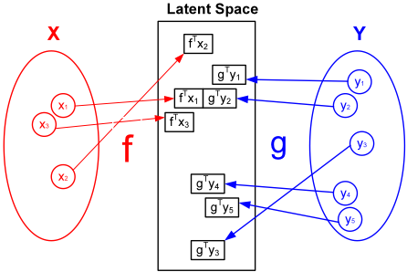
We want to construct a mapping function f for X and g for Y to map both X and Y to a new d dimensional joint (latent) space, where (1) xi and yj are mapped to adjacent locations if they are associated with relation r, (2) xi and yj are mapped to locations away from each other if they are not associated with r, and (3) similar examples within both X and Y will still be close to each other after the mapping. One thing to note is that the terms in argument1 and argument2 sets may not be associated with any existing relation. An illustration of the problem is given in Figure 1.
Using the "birthplace" relation as an example, the term set associated with argument1 contain the names of all the people, and each of them can be represented by features like "age", "occupation", etc. The term set associated with argument2 include all the locations, and each of them can be represented by features like "longitude", "latitude", etc. We will learn mapping functions to project the people set and the location set to one single joint space, matching related terms, separating unrelated terms, and preserving the neighborhood relationship within the original term sets. The new joint space is then used with conventional learning approaches to detect "birthplace" relation from the input term pairs.
3.2 Notation
We first define matrix W to model the nearest neighbor relationship for both X and Y :
where Wx and Wy represent the nearest neighbor graphs (based on Euclidean distance) for X and Y . Wx(i↪ j) = 1 when xi and xj are neighbors; and 0, otherwise. Wy is defined in a similar manner. As a result, Wx is an m⇥m matrix, and Wy is an n⇥n matrix. We also define the corresponding diagonal row sum matrix D as D(i↪ i) = Pj W(i↪ j) and combinatorial Laplacian matrix as L = D - W .
Next, we define the similarity matrix Ws, its row sum matrix Ds, and the corresponding combinatorial Laplacian matrix Ls:
where W x↪y s = (W y↪x s )T is anm⇥nmatrix. W x↪y s (i↪ j) = 1, if relation r is held between xi and yj ; W x↪y s (i↪ j) = 0, otherwise. The corresponding diagonal row sum matrix is defined as Ds(i↪ i) = Pj Ws(i↪ j), and combinatorial graph Laplacian matrix Ls = Ds - Ws.
Dissimilarity matrix Wd (an m ⇥ n matrix), and its corresponding row sum matrix Dd and combinatorial Laplacian matrices Ld are defined in a similar manner:
where W x↪y d = (W y↪x d )T . Wd(i↪ j) = 0, if xi and yj are known to be associated with r; Wd(i↪ j) = 1, otherwise. Dd(i↪ i) = Pj Wd(i↪ j), and Ld = Dd - Wd.
The joint input matrix Z is defined as:
3.3 Objective
We define S1, S2 and S3: functions to be used in the objective.
If xi and xj are similar in their feature space, then the corresponding Wx(i↪ j) will be large. When f T xi and f T xj are well-separated from each other in the new space, S1 becomes large. So minimizing S1 is to preserve the neighborhood relationship of the input datasets. Preserving the neighborhood relationship is particularly useful for scenarios in which similar arguments are often associated with similar relations. This forces similar terms to be projected to adjacent locations in the joint space.
If xi and yj are associated with relation r, but their mapping results are not close to each other, then S2 will be large. Minimizing S2 encourages the related terms to be projected to similar locations in the new space.
If xi and yj are not associated with relation r, but their mapping results are close to each other in the new space, then S3 will be small. So maximizing S3 encourages the unrelated terms to be separated in the new space.
We define the overall cost function Cost(f↪ g) to be minimized as:
where θ is a weight parameter.
3.4 Analysis
Let γ = [f T ↪ gT ]T be a (p+q)⇥d matrix that we want to construct. The solution to minimize Cost(f↪ g) is a special case of [Wang and Mahadevan, 2011] and can be constructed in the following theorem with conventional techniques [Wilks, 1963].
Theorem 1 The γ that minimizes Cost(f↪ g) is given by the eigenvectors corresponding to the smallest non-zero eigenvalues of Z(θL + Ls)Z T ⇠ = λZLdZ T ⇠.
Proof:
When d = 1, it can be verified that:
Based on the Lagrange multiplier method, the γ to minimize Cost(f↪ g) is the eigenvector corresponding to the smallest non-zero eigenvalue of:
Similarly, when d > 1, it can be shown that the γ that minimizes Cost(f↪ g) is given by the eigenvectors corresponding to the d lowest non-zero eigenvalues of
3.5 Feature and Feature Expansions
We use pre-trained term vectors as the input to our model. Typical algorithms to learn term vectors include Latent Semantic Analysis (LSA) [Deerwester et al., 1990] and Word2Vec [Mikolov et al., 2013].
We can also expand these features with domain knowledge like semantic types, etc. Commonly used ontologies containing such domain knowledge include UMLS [Lindberg et al., 1993], and YAGO [Suchanek et al., 2007], etc.
For each relation, all the terms associated with argument1 will be represented by the same features. Similarly, all the terms associated with argument2 will also be represented by the same features. However, the features associated with argument1 can be very different from the features associated with argument2.
After the term xi and yj are projected onto the joint (latent) space using f and g, f T xi and gT yj are directly comparable. To better represent their relationship, we produce several straightforward expansions, including
- ÷ "sum": f T xi + gT yj
- ÷ "difference": ♣f T xi - gT yj♣
- ÷ "product": f T xi · gT yj
3.6 Algorithm
The algorithm to build a detector for relation r with the joint space model has three steps.
1. Construct the mapping functions f and g using Theorem 1.
- ÷ The input to the training algorithm includes X and Y corresponding to the two argument sets associated with r. It also includes a set of term pairs (one fromX, another from Y ) that are known to bear relation r, and a set of term pairs that are known not to bear relation r.
- ÷ One thing to note is that among a total number of m · n term combinations produced by X and Y , only a small number of them are known to "bear" or "not bear" relation r. The labels for others are unknown.
- ÷ L, Ls, Ld and Z are constructed from these input datasets as shown in Section 3.2.
- Project argument sets X and Y to the d dimensional joint space using f and g, resulting in relation specific term embeddings.
- ÷ d is specified by users.
- Use conventional learning techniques to build relation detectors in the joint space (with or without using the feature expansion results constructed in Section 3.5).
- ÷ Our algorithm focuses on the construction of the joint space. In the experiments, we apply a linear SVMmodel on top of the joint space to see how the joint space helps relation extraction.
- ÷ At the test time, the algorithm takes a term pair as the input, uses f and g to map the input to the joint space and then applies the relation detector to the result for relation extraction.
4 Experiments
We used the liblinear package [Fan et al., 2008] as our classifier in the experiments. In all these experiments, the weight for the positive examples was set to 100. All the other parameters were set to the default values. The evaluation of different approaches was based on the F1 scores, where the threshold was chosen to maximize the F1 for the training data.
4.1 Baseline Approaches
Two approaches were used to produce the raw features for each individual term: LSA model [Deerwester et al., 1990] and Word2Vec model [Mikolov et al., 2013]. When we constructed Word2Vec model, the Hierarchical Softmax+CBOW setting was used. The parameters used in training were: window size=5, and sample rate=1e-5. Training the LSA model only required one parameter: desired dimensionality.
Affine matching [Jain, 1986] is a well-known approach to align two datasets with the correspondences. We used affine matching to learn a mapping function to align the argument1 set with the argument2 set. This process also resulted in a single space for both arguments. Another baseline approach used in our experiments was to represent a term pair xi and yj as a vector concatenating the vector representations of both xi and yj . This approach does not require an alignment, since it does not need the input terms to be represented by the same features. RESCAL [Nickel et al., 2011] was our third baseline, where we merged all arg1-relation-arg2 triples into a tensor and used the tensor reconstruction results to judge if a pair of terms bear the desired relation. The last baseline was TransE [Bordes et al., 2013]. In TransE, the learning rate, margin and number of epoches were set to 0.001, 1 and 100. Dimensionality of the latent space was set to 100 for both TRESCAL and TransE.
4.2 Parameters for the Joint Space Model
Once the pre-trained word vectors are given, the joint space can be constructed in a straightforward manner. There are three parameters to specify. The default value of θ is 1, which means S1 and S2 (defined in Section 3.3) will be associated with equal weights. If θ = 0, the neighborhood relationship will not be respected. The default value of k in kNN graph construction is 10. In all experiments, we set the desired dimension of the joint space to be 100, i.e. d = 100.
4.3 DBpedia Relation Extraction
Corpus and Relations
In this experiment, the Wikipedia corpus was used to train LSA and Word2Vec models. The relation data was extracted from DBpedia [Auer et al., 2007], which contains the examples for thousands of different relations in the format of (relation name, argument 1, argument 2). We first filtered out the invalid examples from each relation. A valid example means both argument terms occur at least twice in our corpus. Among all the relations with more than 10K valid examples, we randomly selected 8 of them for our experiment. We generated the argument1 and argument2 term sets by collecting all the argument1 and argument2 terms from the valid examples under each relation.
Training/Test Data
For each relation, about 10K examples were randomly selected from all valid examples as the positive examples. To resemble the real-world challenges, where most of the given term pairs do not bear the desired relation, we randomly generated about 100 times more term pairs as the negative examples by choosing one term from argument1 set and another term from argument2 set. If a generated term pair is known to bear the given relation, it will be removed. Some negative examples generated in this way may still be positives, but this should be rare. We divided both the positive and negative set into 3 parts: 40% as training set 1, 30% as training set 2 and the remaining 30% as the test set. The training set 2 was also used to learn the new joint space in both the proposed approach and affine matching. The list of all 8 relations, the number of examples in both the training and the test set are listed in Table 1.
Using "birthplace" relation as an example, it has about 122K distinct terms in the argument1 set and 16K distinct terms in the argument2 set. About 10K positive examples, and 1.02M negative examples were used in the experiment.
| Number of Training /Test Examples | LSA concate- nated features | word2vec concate- nated features | word2vec affine matching no ex- pansion | Joint Space θ = 0 no ex- pansion | Joint Space θ = 1 no ex- pansion | word2vec affine matching | Joint Space θ = 0 | Joint Space θ = 1 | |
|---|---|---|---|---|---|---|---|---|---|
| birthplace | 720K/308K | 0.3465 | 0.3866 | 0.3935 | 0.3852 | 0.3985 | 0.3739 | 0.3493 | 0.3734 |
| country | 737K/316K | 0.4028 | 0.3641 | 0.3716 | 0.4040 | 0.4425 | 0.4218 | 0.4597 | 0.4206 |
| hometown | 877K/376K | 0.3546 | 0.3315 | 0.3336 | 0.3796 | 0.3818 | 0.3386 | 0.3372 | 0.3601 |
| instrument | 959K/435K | 0.0195 | 0.5295 | 0.5289 | 0.6307 | 0.6176 | 0.5672 | 0.5818 | 0.5847 |
| militarybranch | 765K/353K | 0.3348 | 0.3991 | 0.3998 | 0.4370 | 0.4299 | 0.4152 | 0.4026 | 0.4079 |
| nationality | 1.1M/468K | 0.4759 | 0.4257 | 0.4294 | 0.4760 | 0.4760 | 0.4370 | 0.4416 | 0.4506 |
| occupation | 762K/327K | 0.0292 | 0.2432 | 0.2470 | 0.4095 | 0.3452 | 0.3907 | 0.4372 | 0.3516 |
| religion | 1.2M/525K | 0.3055 | 0.2945 | 0.2887 | 0.3634 | 0.3620 | 0.3259 | 0.3253 | 0.3370 |
| average | 892K/389K | 0.2836 | 0.3718 | 0.3741 | 0.4357 | 0.4317 | 0.4088 | 0.4168 | 0.4107 |
Raw Features and the Joint Space
In LSA related experiments, the raw features to represent each input term were the LSA features (100 dimensional). In Word2Vec related experiments, the raw features were the Word2Vec features (100 dimensional). Joint space models also used the Word2Vec features as the raw input. Affine matching mapped the 100 dimensional raw features associated with argument1 to the feature space of argument2. The classification was then done in the new space. The joint space models constructed a new 100 dimensional joint space, and did relation extraction in that space.
Results
The results are summarized in Table 1. As described in the previous section, in real world applications the number of negative examples is often orders of magnitude more than positive examples which suggests a simple majority baseline will achieve a high accuracy. This makes accuracy a less informative metric, and we decide to focus on F1 score.
From the table, we can see that the LSA model with the concatenated raw features returned the lowest average F1 score of 28▷36%, followed by the Word2Vec model with the concatenated raw features (37▷18%).
When the relation detectors were built from the new joint space, the average F1 scores went up. Under this setting, the new joint space model returned the best score across all approaches (F1 = 43▷57%) and beat the affine matching (F1 = 37▷41%) by a large margin of 6▷16%.
Using the feature expansion results to build classifiers further increased the F1 score for word2vec+affine matching baseline by 3▷4% to 40▷88%. However, it hurt the joint space models by about 2%. Overall, the two joint space models with feature expansions beat all other approaches except the joint space model without using the feature expansions.
From Table 1, we can also see that setting θ = 0 does not make too much difference on F1 scores. The reason for this is that the amount of the training data was large in our experiments (on average, 0.89M for training and 0.389M for testing) and the number of the features was small. Under this situation, overfitting is unlikely to happen.
RESCAL [Nickel et al., 2011] and TransE [Bordes et al.,
2013] did not return satisfying results in this experiment. The average F1 were 3▷35% and 20▷62%. Like most previous KB completion approaches, these two approaches require large amount of labeled positive data (e.g. hundreds of thousands of positive instances), which is not available for our experiments. RESCAL and TransE need to access the training data of all relations during training, so their results are not directly comparable to other approaches, and thus not included in Table 1. We also tested RESCAL and TransE by building a model for each individual relation (rather than a model for all relations) in both DBpedia and Medical experiments, and found the results were worse.
4.4 Medical Relation Extraction
Corpus and Relations
Our medical corpus has incorporated Wikipedia articles and MEDLINE abstracts (2013 version). The relation data used in this experiment was from UMLS [Lindberg et al., 1993]. The UMLS 2012 Release contains more than 600 relations and 50M relation instances under around 15 categories. Each relation has a certain number of Concept Unique Identifier (CUI) pairs that are known to bear that relation. The UMLS consists of a set of 133 subject categories, or semantic types, that provide a consistent categorization of all CUIs. The semantic types can be further grouped into 15 semantic groups.
Following the approach described in [Wang and Fan, 2014], we extracted the UMLS relations corresponding to 6 key medical relations: "treats", "prevents", "causes", "location of", "diagnoses" and "symptom of" and used them to compare different algorithms in our experiments. The UMLS produced a huge amount of the CUI pairs under these 6 relations. However, the majority of them contained the CUIs that are not in our corpus. In this paper, we only consider the relation examples with both CUIs in the corpus.
The arguments of each of these 6 relations are specified by a certain number of semantic types and semantic groups. When we generated the argument1 and argument2 term set for each relation, we extracted all CUIs under the desired types and semantic groups.
| Number of Training /Test Examples | LSA concate- nated features | word2vec concate- nated features | word2vec affine matching no ex- pansion | Joint Space θ = 0 no ex- pansion | Joint Space θ = 1 no ex- pansion | word2vec affine matching | Joint Space θ = 0 | Joint Space θ = 1 | |
|---|---|---|---|---|---|---|---|---|---|
| treats | 461K/198K | 0.2493 | 0.5215 | 0.5223 | 0.6181 | 0.6254 | 0.6756 | 0.7936 | 0.7913 |
| prevents | 63K/27K | 0.2637 | 0.5734 | 0.5699 | 0.5507 | 0.6483 | 0.7661 | 0.6917 | 0.7671 |
| causes | 14K/6K | 0.6596 | 0.4220 | 0.4667 | 0.4706 | 0.4587 | 0.2069 | 0.2697 | 0.4235 |
| location of | 1.26M/539K | 0.3982 | 0.3072 | 0.3111 | 0.4287 | 0.4145 | 0.4762 | 0.6969 | 0.6919 |
| diagnoses | 9K/4K | 0.0370 | 0.5051 | 0.4299 | 0.40000 | 0.4286 | 0.4524 | 0.3226 | 0.3944 |
| symptom of | 865K/371K | 0.1865 | 0.3509 | 0.3417 | 0.4031 | 0.3943 | 0.3711 | 0.5489 | 0.5220 |
| average | 447K/218K | 0.2991 | 0.4467 | 0.4403 | 0.4785 | 0.4950 | 0.4914 | 0.5539 | 0.5984 |
Training/Test Data
The training and test datasets were created in a similar manner as Section 4.3. The only difference was that we used all available relation examples from UMLS, since UMLS did not produce as many relation examples as DBpedia. Table 2 lists the number of examples used in experiments.
Raw Features and the Joint Space
During the corpus preprocessing step, if a term was associated with a CUI, we used the CUI to replace the term. Both the LSA model and the Word2Vec model were applied to the processed corpus, resulting in the vector representations for all the CUIs and other terms in the corpus.
Similar to Section 4.3, in LSA related experiments, the raw features to represent each input term were the LSA features (100 dimensional). In Word2Vec related experiments, the raw features were the Word2Vec features (100 dimensional). Joint space models also used the Word2Vec features as the raw input. Different from the DBpedia experiment, we also expanded the raw feature set by the related semantic type/group information in this experiment. Since the allowed types/groups may be different from relation to relation. The arguments used in different medical relations may be defined by different features. Affine matching models and joint space models were constructed in the same way as Section 4.3.
Results
The results are summarized in Table 2.
One result we can see from the table is that the average F1 scores in the medical relation experiments are significantly better than the scores produced in the DBpedia relation experiments. This is mainly due to the difference between the medical relations and the DBpedia relations. All 6 medical relations are related to diseases, and similar diseases are often associated with similar treatments, causes, symptoms and diagnose methods, etc. Algorithms based on joint spaces fit particularly well for this task. This property may not hold for some DBpedia relations like "birthplace", where the joint space models cannot improve the F1 score in a straightforward manner.
The feature expansions helped both the joint space models and the word2vec+affine matching method. On average, the boost was more than 7% on F1 score. The expanded features can better capture the relationship between term embeddings in the joint space, and helped improve the F1 score. Overall, the two joint space models with feature expansions returned the best F1 scores across all approaches: 59▷84% and 55▷39%, followed by joint space models without feature expansions and word2vec+affine matching. RESCAL returned a result similar to LSA (average F1 = 30▷83%) for this experiment. TransE performed poorly on this set (average F1 = 3%) due to the lack of positive training data.
Another result from Table 2 is that setting θ = 1 significantly helped the joint space model (with feature expansion) when given limited amount of training data. For the three medical relations with least amount of labeled data ("prevents", "causes" and "diagnoses"), including unlabeled instances (i.e. setting θ = 1) improved F1 by approximately 10% each. For the three relations with the most amount of labeled data, there was little improvement. This is because when the labeled data set is small, and if the joint space is learned solely from the labeled data, overfitting will be likely. Setting θ = 1 encourages the neighborhood relationship to be preserved, alleviating overfitting.
5 Conclusions
We present a novel approach for relation extraction using the term pairs as the input. We aim to construct a single joint space for each relation to provide relation specific term embeddings. The joint space associated with each relation is in fact an underlying concept space spanning the relation, and will help remove the redundant information not specific for that relation. The benefits of our approach are three-fold. 1, our approach provides a closed-form solution, which will not suffer from local minimum as many previous works. 2, the proposed method can fit for scenarios in which similar arguments are often associated with similar relations. 3, the proposed approach can handle the situation when the labeled data is limited.
@inproceedings{ijcai2016p417,
  title     = {Building Joint Spaces for Relation Extraction},
  author    = {Wang, Chang and Cao, Liangliang and Fan, James},
  booktitle = {Proceedings of the Twenty-Fifth International Joint Conference on
               Artificial Intelligence, {IJCAI-16}},
  publisher = {AAAI Press / International Joint Conferences on Artificial Intelligence},
  editor    = {Subbarao Kambhampati},
  pages     = {2936--2941},
  year      = {2016},
  month     = {7},
  url       = {https://ijcai.org/proceedings/2016/417},
}
TY - CPAPER TI - Building Joint Spaces for Relation Extraction AU - Wang, Chang AU - Cao, Liangliang AU - Fan, James T2 - Proceedings of the Twenty-Fifth International Joint Conference on Artificial Intelligence, IJCAI-16 PB - AAAI Press / International Joint Conferences on Artificial Intelligence PY - 2016 SP - 2936 EP - 2941 UR - https://ijcai.org/proceedings/2016/417 ER -Copied
Machine-readable versions of this paper, for tools and AI agents:





