
Robust Repositioning to Counter Unpredictable Demand in Bike Sharing Systems
Proceedings of the Twenty-Fifth International Joint Conference on Artificial Intelligence. Pages 3096-3101.
Abstract
Bike Sharing Systems (BSSs) experience a significant loss in customer demand due to starvation (empty base stations precluding bike pickup) or congestion (full base stations precluding bike return). Therefore, BSSs operators reposition bikes between stations with the help of carrier vehicles. Due to unpredictable and dynamically changing nature of the demand, myopic reasoning typically provides a below par performance. We propose an online and robust repositioning approach to minimise the loss in customer demand while considering the possible uncertainty in future demand. Specifically, we develop a scenario generation approach based on an iterative two player game to compute a strategy of repositioning by assuming that the environment can generate a worse demand scenario (out of the feasible demand scenarios) against the current repositioning solution. Extensive computational results from a simulation built on real world data set of bike sharing company demonstrate that our approach can significantly reduce the expected lost demand over the existing benchmark approaches.
- [Battarra et al., 2014] Maria Battarra, Günes Erdogan, and Daniele Vigo. Exact algorithms for the clustered vehi- cle routing problem. Operations Research, 62(1):58-71, 2014.
- [Borgnat et al., 2009] Pierre Borgnat, Patrice Abry, Patrick Flandrin, Jean-Baptiste Rouquier, et al. Studying lyon's vélov: a statistical cyclic model. In European Conference on Complex Systems, 2009.
- [Borgnat et al., 2011] Pierre Borgnat, Patrice Abry, Patrick Flandrin, Céline Robardet, Jean-Baptiste Rouquier, and Eric Fleury. Shared bicycles in a city: A signal process- ing and data analysis perspective. Advances in Complex Systems, 14(03):415-438, 2011.
- [Chemla et al., 2013] Daniel Chemla, Frédéric Meunier, and Roberto Wolfler Calvo. Bike sharing systems: Solving the static rebalancing problem. Discrete Optimization, 10(2):120-146, 2013. Contardo et al., 2012]
- Claudio Contardo, Catherine Morency, and Louis-Martin Rousseau. Balancing a dy- namic public bike-sharing system, volume 4. CIRRELT, 2012.
- [Di Gaspero et al., 2013] Luca Di Gaspero, Andrea Rendl, and Tommaso Urli. A hybrid aco+ cp for balancing bi- cycle sharing systems. In Hybrid Metaheuristics, pages 198-212. Springer, 2013.
- [Di Gaspero et al., 2015] Luca Di Gaspero, Andrea Rendl, and Tommaso Urli. Balancing bike sharing systems with constraint programming. Constraints, pages 1-31, 2015.
- [George and Xia, 2011] David K George and Cathy H Xia. Fleet-sizing and service availability for a vehicle rental system via closed queueing networks. European Journal of Operational Research, 211(1):198-207, 2011.
- [Ghosh and Varakantham, 2016] Supriyo Ghosh and Pradeep Varakantham. Strategic planning for setting up base stations in emergency medical systems. In International Conference on Automated Planning and Scheduling (ICAPS), 2016.
- [Ghosh et al., 2015] Supriyo Ghosh, Pradeep Varakantham, Yossiri Adulyasak, and Patrick Jaillet. Dynamic redeploy- ment to counter congestion or starvation in vehicle sharing systems. In International Conference on Automated Plan- ning and Scheduling (ICAPS), 2015.
- [Kabra et al., 2015] Ashish Kabra, Elena Belavina, and Karan Girotra. Bike-share systems: Accessibility and availability. In Chicago Booth Research Paper, 2015.
- [Leurent, 2012] Fabien Leurent. Modelling a vehicle- sharing station as a dual waiting system: stochastic frame- work and stationary analysis. In Under review, URL https://hal.archivesouvertes.fr/hal-00757228, 2012. Link
- [Lowalekar et al., 2016] Meghna Lowalekar, Pradeep Varakantham, and Patrick Jaillet. Online spatio-temporal matching in stochastic and dynamic domains. In AAAI Conference on Artificial Intelligence (AAAI), 2016.
- [Meddin and DeMaio, 2016] Russell Meddin and Paul DeMaio. The bike-sharing world map. In http://www.bikesharingworld.com/, 2016. Link
- [Nair and Miller-Hooks, 2011] Rahul Nair and Elise Miller- Hooks. Fleet management for vehicle sharing operations. Transportation Science, 45(4):524-540, 2011.
- [Nair et al., 2013] Rahul Nair, Elise Miller-Hooks, Robert C Hampshire, and Ana Bušić. Large-scale vehicle sharing systems: Analysis of vélib'. International Journal of Sus- tainable Transportation, 7(1):85-106, 2013.
- [Pfrommer et al., 2014] J. Pfrommer, J. Warrington, G. Schildbach, and M. Morari. Dynamic vehicle redis- tribution and online price incentives in shared mobility systems. IEEE Transactions on Intelligent Transportation Systems, 15(4):1567-1578, Aug 2014.
- [Rainer-Harbach et al., 2013] Marian Rainer-Harbach, Pet- rina Papazek, Bin Hu, and Günther R Raidl. Balancing bicycle sharing systems: A variable neighborhood search approach. Springer Berlin Heidelberg., 2013.
- [Raviv and Kolka, 2013] Tal Raviv and Ofer Kolka. Opti- mal inventory management of a bike-sharing station. IIE Transactions, 45(10):1077-1093, 2013.
- [Raviv et al., 2013] Tal Raviv, Michal Tzur, and Iris A Forma. Static repositioning in a bike-sharing system: models and solution approaches. EURO Journal on Trans- portation and Logistics, 2(3):187-229, 2013.
- [Saisubramanian et al., 2015] Sandhya Saisubramanian, Pradeep Varakantham, and Lau H. Chuin. Risk based optimization for improving emergency medical systems. In AAAI Conference on Artificial Intelligence (AAAI), 2015.
- [Schuijbroek et al., 2013] Jasper Schuijbroek, Robert Hampshire, and Willem-Jan van Hoeve. Inventory rebal- ancing and vehicle routing in bike sharing systems. In Tech. Rep. 2013-E1, Tepper School of Business, Carnegie Mellon University, 2013.
- [Shu et al., 2013] Jia Shu, Mabel C Chou, Qizhang Liu, Chung-Piaw Teo, and I-Lin Wang. Models for ef- fective deployment and redistribution of bicycles within public bicycle-sharing systems. Operations Research, 61(6):1346-1359, 2013.
References were extracted automatically from the PDF and may contain errors.
Full text extracted automatically from the PDF; figures, tables and equations may differ. The PDF is the version of record.
1 Introduction
Bike Sharing Systems (BSSs) are widely installed in major cities of the world to mitigate the concerns associated with extensive usage of private vehicles such as increased carbon emissions, traffic congestion and usage of non-renewable resources. Because of this ability to provide healthier living and greener environments, bike sharing systems are widely adopted with 984 active systems and 295 systems under construction [Meddin and DeMaio, 2016] in major cities of the world. Popular examples of BSSs include Capital Bikeshare in Washington DC, Hubway in Boston, Bixi in Montreal, and Velib in Paris. In a typical bike sharing system, a set of base stations are strategically placed throughout a city and each of the stations has a finite number of docks, each holding one bike. At the beginning of the day, each station is stocked with a pre-determined number of bikes. Users can hire bikes from one station and return them to a different station.
Pradeep Varakantham
School of Info. Systems Singapore Management Univ. pradeepv@smu.edu.sg
Due to the individualistic and uncoordinated movements of customers, there is often starvation (fewer than required) or congestion (more than required) of bikes at certain base stations, which can result in a significant loss of customer demand. Several bike sharing operators employ carrier vehicles to reposition bikes during the day using myopic reasoning (e.g. start filling when number of bikes falls below 20% of the capacity) to better match the demand. Due to uncertainty in future demand, it is difficult to predict the ideal inventory level and therefore, myopic solutions often fail to provide a good quality solution. While the existing offline multi-step algorithms [Ghosh et al., 2015] based on expected future demand are suitable for situations with stable demand patterns, they perform poorly when demand varies throughout the day. While data driven solution approaches that consider demand uncertainty have been proposed in several application domains (ex: emergency medical services [Saisubramanian et al., 2015; Ghosh and Varakantham, 2016], taxi fleet optimization [Lowalekar et al., 2016]), progress remains slow in handling the unpredictable demand in a robust manner, particularly in bike sharing systems. This serves as the motivation for this paper.
To address such scenarios where demand has high variance, we propose an online and robust repositioning approach to better match the demand and supply of bikes and consequently to reduce the expected lost demand. We treat the problem of computing a robust solution as an iterative game between the decision maker of the BSS and the environment acting as an adversary. In each iteration, the adversary identifies a feasible demand scenario that maximises the lost demand relative to the rebalancing strategy proposed by the decision maker. From the decision maker's perspective, we solve this game using a scenario generation approach. That is to say, the decision maker takes into account all the demand scenarios generated by the adversary in previous iterations and computes a routing and repositioning solution for the vehicles that minimises the worse case lost demand over all the scenarios. The process continues until the objectives of the adversary and the decision maker converges.
We develop an online approach where the robust strategy is generated at each time step by considering the current distribution of bikes across the stations and the strategy is executed on a real world simulator to identify the distribution of bikes for the next time step. Experimental results on multiple synthetic data sets and a real world data set demonstrate that our approach significantly reduces the expected lost demand over the existing benchmark approaches and is robust to the uncertainty in demand.
2 RelatedWork
Given the practical importance of bike sharing systems, they have been studied extensively in the literature. We broadly categorize the repositioning problem into three threads of research. The first thread of research focuses on static repositioning [Chemla et al., 2013] where the goal is to find the routes for a fixed set of vehicles for achieving the desired configuration of bikes across the base stations at the beginning of the day. [Raviv and Kolka, 2013; Raviv et al., 2013; Rainer-Harbach et al., 2013] propose scalable exact and approximate algorithms to solve the static repositioning problem by employing constraints from inventory management literature or by using variable neighborhood search heuristic. [Di Gaspero et al., 2013; 2015] employ constraint programming (CP) and efficiently solve the problem using large neighbourhood search. These notably scalable static repositioning solutions are fruitful if the demand pattern is stable and predictable. However, if the demand changes over time, the stations get imbalanced during the day and static repositioning is not sufficient in those situations. Therefore, our approach focuses on repositioning during the day.
The second thread of research focuses on performing dynamic repositioning of bikes during the day. [Shu et al., 2013] provide an optimisation model for dynamic repositioning to minimise the number of unsatisfied customers. [Ghosh et al., 2015] consider the dynamic repositioning of bikes in conjunction with the routing problem for vehicles. Due to the inherent complexity of the joint problem, they employ decomposition and abstraction based heuristics to solve the real world large scale problems. [Contardo et al., 2012] develop a myopic repositioning approach by considering the recently observed demand to reduce the unmet demand in rush hours. [Pfrommer et al., 2014] provide myopic online decisions based on assessment of near future demand. [Schuijbroek et al., 2013] propose a scalable approximate solution for this problem by abstracting base stations and solving it using a clustered vehicle routing [Battarra et al., 2014] approach. All the papers in this thread assume a known distribution of demand and they are not sensitive to the fluctuating or unpredictable demand scenarios. In contrast, we propose a robust solution approach for the dynamic repositioning problem by considering the possible uncertainly in future demand.
The last thread of research focuses on the prediction and analysis of demand in BSS. [Nair and Miller-Hooks, 2011; Nair et al., 2013] provide service level analysis of BSS using dual-bounded chance constraints. [Leurent, 2012] represent the BSS as a dual markovian waiting system. [Borgnat et al., 2009; 2011] propose the idea of predicting temporal user demand and forecasting that information to users. [George and Xia, 2011; Shu et al., 2013; Kabra et al., 2015] represent the customer arrival process at base stations using Poisson distribution. Due to its simplicity and accuracy in representing random arrival processes, we evaluate the performance of our robust strategies on the demand scenarios generated using Poisson distribution.
3 Model: Bike Sharing System
The generic model for Dynamic Repositioning and Routing Problem with demand Uncertainty (DRRPU) in BSS is formally defined using the following tuple:
S represents the set of base stations, where each station s 2 S has a fixed capacity (number of docks) denoted by C # s . V represents the set of vehicles and each vehicle v 2 V has a fixed capacity (number of slots for bikes) denoted by C ⇤ v . The number of bikes stocked at a base station, s at the beginning of the day, is given by d#↪0 s . d⇤↪0 v denotes the number of bikes present initially in a vehicle v. σ0 v (s) is set to 1 if vehicle v is present at station s initially. For ease of notation, we use the generic σtv (s) and set it to 0, if t > 0. Ps↪s0 represents the distance between station s and s0 .
F represents the set of demand bounds that is computed from the historical trip data. We compute three types of bounds on the arrival customer demand: (a) ˇ F t ↪ ˆ F t denote the lower and upper bound on the system wide demand across all the stations at time step t; (b) ˇ F t s ↪ ˆ F t s denote the bounds on the demand in station s at time step t; (c) ˇ F t s↪s0 ↪ ˆ F t s↪s0 denote the bounds on the demand that arises in station s at time step t and reach station s0 at time step t+1. These demand bounds are used in the solution approach to generate the strategy. On the other hand, the strategies are evaluated on a wide range of testing demand scenarios that are created using Poisson distribution and these scenarios are not forced to follow the bounds used in the planning process.
Given the DRRPU model, our goal is to provide a repositioning and routing strategy for the vehicles at each time step that minimises the worse case lost demand. We are primarily interested in minimising lost demand that arises because of the starvation of bikes at stations. As we compute the strategy for one time step, we have no control over the lost demand that arises due to the congestion of bikes at the destination station (which depends on the unknown demand) in the next time step. However, experimental results on the real world data set demonstrate that repositioning bikes to reduce the lost demand at the time of hiring, determine the inventory level efficiently and furthermore, reduce the number of unsatisfied customers at the return time.
4 Solution approach
We compute a robust repositioning and routing strategy using rolling horizon framework. In each decision epoch, for a given distribution of bikes at stations, we compute a robust strategy by assuming that the arrival demand in each station and in aggregate follows the input bounds. Once we obtain the repositioning strategy for a decision epoch, we simulate the customer flows for the given demand scenario along with the repositioning numbers to achieve the distribution of bikes across stations for the next decision epoch. This iterative process continues until we reach the last decision epoch.
For the ease of representation, we made three key assumptions: (a) Customers complete their trips in one decision epoch. That is to say, customers who hire bikes at decision epoch t should return their bikes to the destination station at the beginning of the decision epoch t + 1; (b) Customers are impatient in nature and leave the system if they encounter an empty station. On the other hand, they return their bikes to the nearest available station if the destination station is full; (c) The events at each time step follow a particular sequence. First, the customers return their bikes which was hired in the previous time step, then the repositioning events by the vehicles are done and lastly, the arrival customers hire bikes.
| Variable | Definition |
|---|---|
| y+↪t s↪v | Number of bikes picked up from station s by vehicle v at time index t |
| y-↪t s↪v | Number of bikes dropped off at station s by vehicle v at time index t |
| zts↪s0 ↪v | Set to 1 if vehicle v has to move from station s to s0 at time index t |
| d⇤↪t v | Number of bikes in vehicle v at time index t |
| F k s↪s0 | Arrival customer demand from station s to s0 for kth demand scenario |
To compute a robust strategy in each decision epoch, we propose an iterative two player game approach between the repositioning planner and an adversary. We provide two novel Mixed Integer Linear Programming (MILP) formulations to represent the planning problem for the adversary and the repositioning planner. For ease of understanding, the decision variables employed in the MILP are provided in Table (1).
4.1 The Adversarial Planner
Once the intentions of the repositioning planner are revealed, the adversary aims at providing the worst possible demand scenario that results in lowest bike usage during the planning period. More specifically, the goal is to find a demand scenario that maximises the amount of lost demand, while ensuring constraints related to demand feasibility. In the first iteration the adversary finds a worse demand scenario with the assumption of no repositioning in the system. In the subsequent iterations, the adversary plans against a particular repositioning strategy that is proposed by the repositioning planner. The MILP for the demand selection process by the adversary is shown compactly in Table (2). The inputs for the MILP are the current repositioning strategy, i.e., the number of bikes to pickup, Y + s and drop-off, Y - s at station s. The distribution of bikes, d#↪t s at station s and in the decision epoch t is also provided as input. Let Ls denotes the number of lost demand occurred at station s during the planning period. Fs↪s0 denotes the number of customers arrived in station s at the current decision epoch and reach station s0 at the beginning of the next decision epoch.
The objective delineated in expression (1) is to generate a demand scenario, F that maximises the total amount of lost demand over all the stations. The number of bikes present at station s after the repositioning event can be computed as
Table 2: ADVERSARY(Y +↪ Y -↪ t↪ d#↪drrpu)
(d#s +Y - s -Y + s ). Therefore, constraints (2) compute the lost demand at station s as the deficiency between the demand for bikes (i.e., Ps0 Fs↪s0 ) and the supply of bikes. These constraints are non-linear in nature and we linearise them with a set of inequality constraints using the well known Big-M method. Constraints (3-5) ensure that the generated demand follows the given input bounds. Specifically, constraints (3) ensure that the aggregated system wide demand at the decision epoch t is bounded by ˇ F t and ˆ F t . Constraints (4) enforce that the arrival demand in station s at decision epoch t is bounded by ˇ F t s and ˆ F t s . Constraints (5) enforce that the demand arises in station s at decision epoch t and reach station s0 in the next decision epoch is bounded by ˇ F t s↪s0 and ˆ F t s↪s0 .
4.2 The Repositioning Planner
Given a set of K demand scenarios (computed by the adversary in K iterations), the goal of the repositioning planner is to find the best routing and repositioning strategy for the vehicles that maximises the bike usage or alternatively, minimises the worse case lost demand. Let F k s↪s0 denotes the arrival demand from station s to s0 for scenario k. Lks denotes the lost demand at station s for scenario k. The outcome of the repositioning planner is two-fold: (a) A set of decisions z for the vehicle routes; (b) The repositioning strategy y+ and y- .
The MILP for solving the joint problem of routing and repositioning is represented compactly in Table (3). The objective function delineated in expression (8) is to minimise the maximum lost demand over all the scenarios. We further simplify the objective function by introducing an additional set of constraints (7) to ensure that the total lost demand for scenario k is bounded by the variable λ and we minimise λ in objective function (6).
Note that a vehicle can visit multiple stations in one decision epoch. Let a vehicle visit a maximum of ˆ T number of stations within one decision epoch. To represent the sequence of moves, we use a time index ˆ t 2 [0↪ ˆ T]. After repositioning, the number of bikes present at station s in the decision epoch t can be computed as (d#↪t s +Pˆ t↪v (y-↪ˆ t s↪v -y+↪ˆ t s↪v )). Therefore, constraints (9) ensure that the lost demand at station s for scenario k is equal to the difference between the total arrival demand (i.e., Ps0 F k s↪s0 ) and the supply of bikes. Constraints (10) ensure that the total number of bikes picked up from a station s during the planning period is less than the available bikes, d#↪t s . Constraints (11) enforce that the total number of bikes dropped off at station s is less than the number of available docks, C # s -d#↪t s .
Table 3: REDEPLOYMENT(F,k,t,d#,drrpu)
The initial distribution of bikes in vehicles, d⇤↪0 and the initial distribution of vehicles at stations, σ0 are computed from the state of the system at the end of previous decision epoch. Constraints (12) ensure the flow conservation of bikes in the vehicle. The number of bikes present in vehicle v at time index ˆ t + 1 (i.e., d⇤↪ˆ t+1 v ) is equivalent to the number of bikes present in the vehicle at time index ˆ t (i.e., d⇤↪ˆ t v ) plus the net incoming bikes at time index ˆ t. Constraints (13) enforce the flow conservation of vehicles at stations by ensuring the equivalence between the inflow and outflow of vehicles in each station. For ˆ t = 0, depending on the initial location of vehicles, σ0 v these constraints ensure that vehicles move appropriately out of the initial locations. Constraints (14) enforce that the number of bikes picked up or dropped off is conditional to the station being visited at that time index. Let ↵ denotes the unit for converting distance to time, M denotes the time required to pickup/drop-off one bike and Q denotes the duration of planning period. Then, constraints (15) enforce the physical limitation of the carrier routes. That is to say, total time spent by the vehicles for traveling between the stations plus the time spend on picking up or dropping off the bikes, is bounded by the duration of the planning period. Finally, constraints (16) enforce that the number of bikes picked
Algorithm 1: solveDRRPU(drrpu↪ t↪ d#) 1 Initialize: F ¶♦↪Y+0 ↪Y-0 0↪ i 0 ; 2 repeat 3 i i + 1; 4 Oa↪ Fi ADVERSARY(Y+i-1 ↪Y-i-1 ↪ t↪ d#↪ drrpu) 5 F F[Fi 6 Or↪ zi↪Y-i ↪Y+i REDEPLOYMENT(F↪ i↪ t↪ d#↪ drrpu) 7 until Converge; 8 return y+i ↪ y-i ↪ ziup or dropped off is bounded by the capacity of vehicles.
To better understand the robust optimisation approach, we provide the key iterative steps in Algorithm (1). The repositioning strategies are initialised as 0, therefore, in the first iteration adversary computes a demand scenario against the no repositioning strategy. From the subsequent iteration, the adversary generates a worse demand scenario against the repositioning strategy revealed by the repositioning planner. At iteration k, the repositioning planner has k demand scenarios (communicated by the adversary) and it computes a repositioning strategy that minimises the worse case lost demand over all the scenarios. The process stops when the objectives of the repositioning planner, Or and the adversary, Oa converge. Therefore, at the convergence, the solution guarantees to provide an upper bound on the lost demand for any possible demand scenario that follows the given bounds.
4.3 SimulationModel
We employ the solveDRRPU procedure from Algorithm (1) to compute a repositioning strategy at each time step and execute the strategy on a simulator for the evaluation. Let f t s↪s0 denotes the number of arrival customers in station s at time step t and want to reach station s0 at the beginning of time step t+1. d#↪t s denotes the number of bikes present in station s at time step t after the repositioning is done. The flow of bikes is determined based on the following two cases: (a) If the arrival demand at a station is less than the number of bikes present in the station, then all the customers are served. (b) If the arrival demand at a station is higher than the number of bikes present in the station, then actual flow (denoted as
Once we determine the flow of bikes between stations at time step t, we can compute the distribution of bikes at a station at time step t+1 as the sum of un-hired bikes at time step t, net incoming bikes at the beginning of time step t+1 and the net drop-off bikes by vehicles at time step t + 1.
If the number of bikes in station s at time step t+1, d#↪t+1 s exceeds the station capacity, C # s thenwe transfer the extra bikes
(i.e., d#↪t+1 s -C # s ) to the nearest station to ensure the capacity constraints of the stations. These extra numbers are shown as the lost demand at the time of return in the experimental results. Once we obtain the distribution of bikes across the stations for time step t + 1, this information can readily be utilised to compute the repositioning strategy for time step t + 1. This iterative process continues until we reach the last time step.
5 Experimental Settings
We evaluate our approach with respect to key performance metric of loss in demand, on real world 1 and synthetic data sets. The real world data sets contain the following data: (1) Customer trip records, from which we estimate the bounds on demand; (2) The number of stations, their capacity and initial distribution of bikes in each of the stations; (3) Geographical locations of base stations, from which we calculate the distance between two stations; (4) The number of vehicles and their capacity. We generate the synthetic data sets as follows: (a) We take a subset of the stations from the real world data set (b) Station capacity, their geographical locations and initial distribution of bikes are drawn from the real world data for those specific stations. (c) We generate the demand bounds manually. More specific details on the demand bounds are mentioned later. We compare the utility of our approaches with three existing benchmark approaches as mentioned bellow.
Benchmark-1: Static Repositioning implies the practice of no repositioning during the day. The stations are rebalanced at the end of the day to achieve a predefined inventory level. We use this as a baseline approach where no repositioning is done during the planning period.
Benchmark-2: Myopic Repositioning entails that bikes are repositioned at each time step to reach a certain inventory level. Through the personal communication with bike sharing operators, we infer that 50% of the station capacity is the ideal inventory level and some operators rebalance the stations in a myopic fashion (without considering the demand patterns) to reach that specific inventory level.
Benchmark-3: Online Heuristic is adapted from [Schuijbroek et al., 2013]. This static repositioning approach can be executed online due to its assumption of negligible customer movements during the rebalancing period. As we evaluate the strategies on the demand scenarios generated using Poisson distribution with a known mean, the goal of the online heuristic is to bound the inventory level within 10% of the Poisson mean, while ensuring the physical limitations of the vehicle routes.
To ensure a fair comparison, all the three benchmark approaches and our robust strategy are evaluated by employing a simulation model as described in section (4.3). Furthermore, we compute an upper bound on the optimal solution for the synthetic data sets where exact future demand for the entire horizon is assumed to be known. We employ an MILP formulation proposed by [Ghosh et al., 2015] to compute the optimal solution.
1 Data is taken from Hubway bike sharing company of Boston [http://hubwaydatachallenge.org/trip-history-data]
| Static | Myopic | Online | Robust | Offline | |
|---|---|---|---|---|---|
| MEAN | 822 | 758 | 641 | 638 | 451 |
| STDEV | 37 | 47 | 38 | 38 | 38 |
| MAX | 938 | 908 | 713 | 730 | 521 |
| (a) Scenarios for Uniform Data (data set: 1) | |||||
| MEAN | 956 | 769 | 734 | 704 | 491 |
| STDEV | 48 | 62 | 45 | 48 | 39 |
| MAX (b) | 1069 Scenarios | 974 for Two-Peaked | 825 Data | 826 (data set: | 568 2) |
6 Empirical Evaluation
We report 2 results on two synthetic data sets. Both the data sets consist of 20 stations and 1 vehicle. We generate demand for 14 time steps. Figure 1(a) shows the demand patterns for both the synthetic data sets. We generate the aggregated mean demand at each time step for first data set randomly, while the aggregated mean demand for second data set follows a realistic pattern with two peak hours. For both the data sets, we compute the lower bound on the arrival demand as (1-✏) of the mean demand and upper bound as (1+✏) of the mean demand. To compute the bounds on arrival demand for each station and for each origin destination pair we set ✏ as 100%, while for the bounds on the system wide demand at each time step, ✏ is set as 10%.
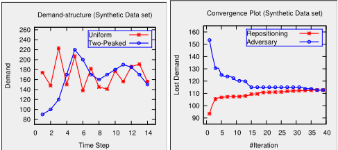
Figure 1(b) shows the convergence of our scenario generation approach on synthetic data. As expected, the gap between the objectives of the adversary and the repositioning planner reduces monotonically and converges after 40 iterations. As both the objectives converge to 112, we can claim that the worse case lost demand is bounded by 112 if the robust strategy is adopted.
To compare the utility of our policy with the existing benchmark approaches, we generate 100 testing demand scenarios, where demand from station s to s0 at time step t, f t s↪s0 is generated using Poisson distribution with known mean parameters. We report average performance statistics in terms of mean, standard deviation and the worse case lost demand over 100 demand scenarios. The performance statistics for the synthetic data set with uniform patterns are demonstrated in Table 4(a). Our approach reduces the average lost demand by 22% over the static approach and by 15% over the myopic approach and is highly competitive with the online approach. Similar performance statistics for the synthetic data set with 2 peak hours are shown in Table 4(b). The average performance of our approach is significantly better than all the three benchmark approaches, which verify the fact that our approach is able to better handle the lost demand at rush hours. More interestingly, the competitive ratio for our solution is approximately 70% of the optimal solution for both the data sets.
2 All the linear optimisation models were solved using IBM ILOG CPLEX Optimisation Studio V12.5 on a 3.2 GHz Intel Core
i5 machine with 8GB DDR3 RAM
| Lost demand at Issue Time | Lost demand at Return Time | |||||||
|---|---|---|---|---|---|---|---|---|
| Static | Myopic | Online | Robust | Static | Myopic | Online | Robust | |
| MEAN | 267 | 269 | 257 | 197 | 61 | 138 | 46 | 50 |
| STDEV | 79 | 77 | 82 | 68 | 19 | 32 | 18 | 15 |
| MAX | 460 | 471 | 453 | 393 | 103 | 196 | 91 | 96 |
| (a) Demand scenarios from real-world data | ||||||||
| MEAN | 145 | 155 | 146 | 100 | 53 | 126 | 37 | 33 |
| STDEV | 18 | 19 | 19 | 18 | 9 | 21 | 14 | 10 |
| MAX | 193 | 202 | 192 | 137 | 83 | 165 | 68 | 74 |
| (b) Demand scenarios follow Poisson distribution at each station | ||||||||
| MEAN | 163 | 171 | 154 | 113 | 69 | 143 | 50 | 54 |
| STDEV | 24 | 22 | 17 | 19 | 13 | 28 | 16 | 14 |
| MAX | 206 | 220 | 204 | 158 | 103 | 208 | 86 | 85 |
| (c) Demand scenarios follow Poisson distribution for each OD pair | ||||||||
Results on the Hubway data set: The next thread of results demonstrate the performance statistics on the Hubway data set. The Hubway BSS consists of 95 base stations and 3 vehicles. We consider a planning horizon of 6 hours in the morning peak (6AM-12PM) and the duration of each decision epoch is 30 minutes. We compute the bounds on demand from three months of historical trip data. As the historical trip data only contains successful bookings and does not capture the unobserved lost demand, we employ a microsimulation model with 1 minute of time step to identify the duration when a station got empty and introduce artificial demand at the empty station based on the observed demand at that station in previous time step.
We produce three threads of demand scenarios (1) We took the real demand data for 60 weekdays. We estimate the actual demand by introducing artificial demand at empty stations using a similar heuristic mechanism discussed earlier; (2) We generate 100 demand scenarios, where the arrival demand at each station is generated using Poisson distribution with the mean computed from historical data. Similar to [Shu et al., 2013], we assume that customers reach their destination station with a fixed probability; (3) We generate 100 demand scenarios, where the demand for each origin destination pair at each time step is computed using Poisson distribution.
For all the three settings of demand scenarios, we summarise the key performance statistics for all the approaches in Table (5). As the planning period for one decision epoch is 30 minutes, we set a time threshold of 3 minutes as a convergence criterion for our scenario generation approach. We provide statistics for two types of lost demand: (a) Lost demand occurred at the time of hiring the bikes due to starvation of bikes at stations; (b) Lost demand occurred at the time of returning the bikes due to the congestion of bikes at stations.
The performance statistics for real demand scenarios are demonstrated in Table 5(a). On an average our approach reduces the overall lost demand by atleast 18% over all the benchmark approaches. Moreover, our approach reduces the worse case lost demand by atleast 10%, hence, is robust to the uncertainty in demand. Similar performance statistics for other two settings of demand scenarios are shown in Table 5(b) and 5(c). For both the settings, the average and worse case performance of our approach is noticeably better than all the three benchmark approaches. The average lost demand is reduced by atleast 27% and 18%, while the worse case lost demand is decreased by atleast 19% and 16%, over all the three benchmark approaches.
7 Conclusion
We develop a robust optimisation approach to solve the dynamic repositioning problem in bike sharing systems. We propose an iterative scenario generation approach where an adversary identifies the worse demand scenario for a given repositioning strategy and the decision maker computes a repositioning strategy by considering a set of demand scenarios proposed by the adversary. The empirical results on a real world and multiple synthetic data sets shown that our approach outperforms the existing benchmark approaches in terms of reducing the expected and worse case lost demand and therefore, improves the operational efficiency of the bike sharing company. In future, this work can be extended with multi-step planning by considering the expected future demand bounds for multiple epochs to better account for the future demand surges. Furthermore, a decomposition technique can be employed for the repositioning planner to scale up the solution process for problems with thousands of stations.
Acknowledgement
This research is supported by the National Research Foundation, Prime Minister's Office, Singapore under its International Research Centres in Singapore Funding Initiative.
@inproceedings{ijcai2016p439,
  title     = {Robust Repositioning to Counter Unpredictable Demand in Bike Sharing Systems},
  author    = {Ghosh, Supriyo and Trick, Michael A. and Varakantham, Pradeep},
  booktitle = {Proceedings of the Twenty-Fifth International Joint Conference on
               Artificial Intelligence, {IJCAI-16}},
  publisher = {AAAI Press / International Joint Conferences on Artificial Intelligence},
  editor    = {Subbarao Kambhampati},
  pages     = {3096--3101},
  year      = {2016},
  month     = {7},
  url       = {https://ijcai.org/proceedings/2016/439},
}
TY - CPAPER TI - Robust Repositioning to Counter Unpredictable Demand in Bike Sharing Systems AU - Ghosh, Supriyo AU - Trick, Michael A. AU - Varakantham, Pradeep T2 - Proceedings of the Twenty-Fifth International Joint Conference on Artificial Intelligence, IJCAI-16 PB - AAAI Press / International Joint Conferences on Artificial Intelligence PY - 2016 SP - 3096 EP - 3101 UR - https://ijcai.org/proceedings/2016/439 ER -Copied
Machine-readable versions of this paper, for tools and AI agents:





