Generalizing the Edge-Finder Rule for the Cumulative Constraint

1 Introduction

Scheduling consists of deciding when a set of tasks needs to be executed on a shared resource. Applications can be found in economics [Buyya et al., 2005] or in industrial sequencing [Harjunkoski et al., 2014].

Constraint programming is an efficient way to solve scheduling problems. Many powerful filtering algorithms that prune the search space have been introduced for various scheduling problems [Baptiste et al., 2001]. These algorithms are particularly adapted for the cumulative problem in which multiple tasks can be simultaneously executed on a cumulative resource. Among these algorithms, we note the Time-Table [Beldiceanu and Carlsson, 2002], the Energetic Reasoning [Lopez and Esquirol, 1996], the Overload Check [Wolf and Schrader, 2006], the Edge-Finder [Mercier and Van Hentenryck, 2008] and the Time-Table Edge-Finder [Vil´ım, 2011].

Constraint solvers call filtering algorithms multiple times during the search, hence the need for them to be fast and efficient. Cumulative scheduling problems being NP-Hard, these algorithms rely on a relaxation of the problem in order to be executed in polynomial time. In this paper, we introduce a novel relaxation that grants a stronger filtering when applied in conjunction with known filtering algorithms.

In the next section, we formally define what a Cumulative Scheduling Problem (CuSP) is. Then, we present two

Claude-Guy Quimper

Universit´e Laval, Qu´ebec, QC, Canada Claude-Guy.Quimper@ift.ulaval.ca

state-of-the-art filtering rules: the Overload Check and EdgeFinder. We generalize these rules so that they become function of the earliest completion time of a set of tasks. We introduce a novel function computing an optimistic value of earliest completion time for a set of tasks, based on a more realistic relaxation of the CuSP. Along with this function, we present a novel data structure, named Profile, we use to compute the function. We introduce two algorithms to enforce the generalized rules while using our own novel function. Finally, we present experimental results obtained while solving CuSP instances from two different benchmark suites.

2 The Cumulative Scheduling Problem

We consider the scheduling problem where a given set of tasks I = ¶1↪ ▷ ▷ ▷ ↪ n♦ must be executed, without interruption, on a cumulative resource of capacity C. A task i 2 I has an earliest starting time esti 2 Z, a latest completion time lcti 2 Z, a processing time pi 2 Z+, and a resource consumption value, commonly referred as height, hi 2 Z+. The energy of a task i is given by ei = pihi. We denote the earliest completion time of a task ecti = esti +pi and the latest starting time lsti = lcti -pi. Some of these parameters can be generalized for a set of tasks ⌦ ✓ I.

Let Si be the starting time of task i, and its domain be dom(Si) = [esti↪ lsti]. The constraint CUMULATIVE([S1↪ ▷ ▷ ▷ ↪ Sn]↪C) is satisfied if the total resource consumption of the tasks executing at any time t does not exceed the resource capacity C, which is expressed as :

A solution to the CUMULATIVE constraint is a solution to the Cumulative Scheduling Problem (CuSP). In addition to satisfying the CUMULATIVE constraint, one usually aims at optimizing an objective function, such as minimizing the makespan, i.e. the time at which all tasks are completed.

Such scheduling problems are NP-Hard [Garey and Johnson, 1979], therefore it is NP-Hard to remove every inconsistent values from the domains of the starting time variables Si. However, there exist many powerful filtering algorithms running in polynomial time for the CUMULATIVE constraint. To execute in polynomial time, these algorithms rely on a relaxation of the original problem that generally revolves around a task property referred as the elasticity [Baptiste et al., 2001]. A task i becomes fully elastic if we allow its resource consumption to fluctuate (and even to interrupt), as long as the amount of resource consumed in the interval [esti↪ lcti) is equal to its energy ei.

3 Preliminaries

We present two filtering algorithms based on an energetic relaxation that we later improve using a novel relaxation.

3.1 Overload Check

The Overload Check is a test that detects inconsistencies in the problem and triggers backtracks in the search tree. The Overload Check rule enforces the condition that the energy consumption required by a set of tasks ⌦ cannot exceed the resource capacity over the time interval [est⌦↪ lct⌦).

This condition is necessary to the existence of a feasible solution to the problem. [Wolf and Schrader, 2006] present an algorithm enforcing this rule running in O(n logn) time. More recently, [Fahimi and Quimper, 2014] presented an Overload Check algorithm that runs in O(n) time, using a data structure named Timeline. Although initially conceived for the DISJUNCTIVE constraint, it is demonstrated that the algorihtm can be adapted for the CUMULATIVE constraint, while maintaining its running time complexity of O(n).

3.2 Edge-Finder

The Edge-Finder algorithm filters the starting time variables. The algorithms by [Vil´ım, 2009] and [Kameugne et al., 2014] proceed in two phases : the detection and the adjustment.

The detection phase detects end before end temporal relations between the tasks. The relation ⌦<· i indicates that the task i must finish after all tasks in ⌦ are completed.

Given a set of tasks ⌦ ✓ I, the Edge-Finder detection rule enforces the condition that if a task i 62 ⌦ cannot be concurrently executed along the tasks in ⌦ without having any of themmissing their deadline, then the tasks in ⌦must end before the task i ends, i.e. ⌦<· i. [Baptiste et al., 2001] present the following rule.

[Vil´ım, 2009] detects all precedences using this rule. He demonstrates that the rule does not require to be applied for all subsets. Let the left cut of task i be the set of tasks whose lct is no greater than lcti, i.e. LCut(I↪ i) = ¶j 2 I ♣ lctj  lcti♦. Then the algorithm only needs to enforce the rule (3) for all distinct left cuts. Additionally, Vil´ım's detection algorithm introduces the ⇥-⇤-tree data structure to achieve a O(n log n) time complexity.

Assuming a precedence relation ⌦<· i is found during the detection phase, the adjustment phase proceeds to filter the earliest starting time of task i. The new value is computed by spending the energy e⌦ in the time interval [est⌦↪ lct⌦) as follows. A maximum amount of energy is spent on the interval with a restricted capacity of C - hi. The remaining energy, i.e. max(0↪ e⌦ - (lct⌦ -est⌦)(C - hi)), is spent as early as possible on the interval using the remaining capacity hi. The time when this remaining energy completes its execution is the new bound esti. [Baptiste et al., 2001] present the following rule for the adjustment phase.

The main difficulty of the adjustment phase is to compute the subset ⌦0 that results in the optimal adjustment. [Vil´ım, 2009] introduces an adjustment algorithm running in O(kn logn) time, where k is the number of distinct heights. His algorithm uses an extended ⇥-⇤-tree. In an orthogonal work, [Kameugne et al., 2014] introduce an adjustment algorithm running in O(n2 ) time, based on notions of minimum slack and maximum density. Although their algorithm does not strictly dominate Vil´ım's algorithm complexity, they demonstrate that it performs better in practice.

4 Novel function of earliest completion time

The earliest completion time of a set of tasks ⌦, denoted ect⌦, is NP-Hard to compute [Garey and Johnson, 1979]. One normally uses a relaxation in order to compute an optimistic (smaller) value of earliest completion time. This relaxation can be identified as the fully-elastic relaxation [Baptiste et al., 2001]. In order to differentiate the two functions of ect presented in this paper, we took the discretion to rename the function of ect presented by [Vil´ım, 2009] as ectF. It is computed by spending a maximum amount of energy as early as possible without any regards to the heights of the tasks. [Vil´ım, 2009] uses the following formula to compute it.

We introduce a generalization of the Overload Check rule based on the function ect or any of its relaxation. If a particular set of tasks cannot be completed before the deadline of this set, then the problem does not have a solution.

Substituting the function ect by the fully-elastic relaxed ectF (5) into rule (6) leads to the well known form of the Overload Check rule (2). The demonstration follows from inequalities (7)-(10) being equivalent.

However, since ectF⌦  ect⌦, rule (6) detects more failure cases than its fully-elastic relaxed version. This suggests to find stronger relaxations for the function ect than ectF.

From [Vil´ım, 2009], we generalize the Edge-Finder detection rule. A precedence is detected when a set of tasks ⌦, executing along a task i 62 ⌦, cannot meet its deadline.

Since computing ect⌦ is NP-Hard, one needs to use a relaxation. The fully-elastic relaxation results in rule (3). The demonstration is similar to the one for the Overload Check.

We introduce a stronger relaxation for the function ect that we call horizontally-elastic. With this relaxation, a task i is allowed to consume, at any time t 2 [esti↪ lcti), between 0 and hi units of resource. Unlike the fully-elastic relaxation, it cannot consume more than hi units of resource. Given a set of tasks ⌦, ectH⌦ is computed using the following formulas.

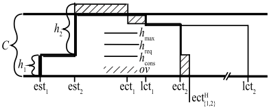
Let hmax(t) represent the amount of resource that can be allocated to the tasks in ⌦ at time t. A task i can consume at most hi units of resource at any time in its execution window [esti↪ lcti). The resource has a capacity C.

Let hreq(t) be the amount of resource required at time t by the tasks in ⌦ if they were all starting at their earliest starting times. In this context, a task i consumes hi units of resource throughout the interval [esti↪ ecti).

We call overflow ov(t) the energy from hreq(t) that cannot be executed at time t due to the limited capacity hmax(t). This overflow is accumulated over time and released when the resource is no longer saturated. Let hcons(t) be the amount of resource that is actually consumed at time t. This amount is given by hreq(t) to which we add the previously accumulated overflow. The resource consumed is limited by hmax(t).

The earliest completion time occurs when all tasks are completed. Figure 1 shows the distribution of the energy along the time line.

Theorem 1 shows that the horizontally-elastic relaxation is stronger than the fully-elastic one.

Proof. The fully-elastic relaxation requires a task i to consume ei units of resource within the interval [esti↪ lcti). The horizontally-elastic relaxation has the same constraint with the added restriction that no more than hi units of resource should be consumed at any given time, which can only make a schedule finish later, hence ectF⌦  ectH⌦ . In the CuSP, a task must consume either 0 or hi units of resource at time t 2 [esti↪ lcti). Morever, there is no interruption. These conditions are even stronger, hence ectH⌦  ect⌦. ⇤

Theorem 2. The Overload Check and Edge-Finder based on the horizontally-elastic relaxation detect a superset of inconsistencies and precedences than their respective version based on the fully-elastic relaxation.

Proof. Since ectF⌦  ectH⌦ for all ⌦ (Theorem 1), the fail condition ectF⌦ > lct⌦ implies the fail condition ectH⌦ > lct⌦. Similarly, ectF⌦[¶i♦ > lct⌦ implies the detection condition ectH⌦[¶i♦ > lct⌦. Consider the instance with C = 2 and four tasks whose parameters hesti↪ lcti↪ pi↪ hii are h0↪ 4↪ 2↪ 1i, h1↪ 4↪ 1↪ 2i, h1↪ 4↪ 1↪ 2i, and h1↪ 4↪ 1↪ 2i. Only the Overload Check based on the horizontally-elastic relaxation fails. In the instance with C = 2 and the tasks x : h0↪ 5↪ 2↪ 1i, y : h1↪ 5↪ 2↪ 1i, z : h1↪ 5↪ 2↪ 2i, and w : h1↪ 10↪ 2↪ 1i. The precedence ¶x↪ y↪ z♦ <· w is only detected when using the horizontally-elastic relaxation. ⇤

5 Resource Utilization Profile

To efficiently compute ectH, we introduce a data structure called Resource Utilization Profile, or simply Profile, that stores the resource utilization over time, as in Figure 1. Similarly to [Gay et al., 2015], we represent the Profile as an aggregation of juxtaposed rectangles of different lengths and heights. Rectangles are expressed with tuples htime↪ capacity↪∆max↪∆reqi, where time is the start time, capacity is the remaining capacity of the resource at the start time, ∆maxand ∆reqare two quantities initialized to zero. The ending time is the starting time of the next rectangle. These tuples are stored in a sorted linked list whose nodes are called time points, referring to the starting times of the rectangles. The Profile is initialized with a time point of capacity C for every distinct value of est, ect and lct. We add a sufficiently large time point to act as sentinel. Finally, while initializing the data structure, pointers are kept so that Testi , Tecti , and Tlcti return the time point associated to esti, ecti, and lcti.

The algorithm ScheduleTasks proceeds in batch to schedule a set of tasks ⇥ on the profile P. The algorithm computes the functions hreq(t), hmax(t), hcons(t), and ov(t). To ensure a strongly polynomial running time complexity, the algorithm does not process indiviual time points, but time intervals for which the functions do not fluctuate. Line 23 sets the remaining capacity of a time point to the capacity of the resource minus the consumed capacity hcons. For future uses, line 11 stores the overflow at the moment of processing the time point and line 32 resets this overflow to the minimum overflow encountered in later time points.

Algorithm 1: ScheduleTasks(⇥↪ c) for all time point t do t▷∆max 0, t▷∆req 0 2 for i 2 ⇥ do 4 Increment Testi ▷∆max and Testi ▷∆req by hi 5 Decrement Tlcti ▷∆max and Tecti ▷∆req by hi 6 t P▷first, ov 0, ect -1, S 0, hreq 0 7 while t▷time 6= lct⇥ do 9 t▷ov ov 11 l t▷next.time - t▷time 12 S S + t▷∆max 13 hmax max(S↪ c) 14 hreq hreq + t▷∆req 15 hcons min (hreq + ov↪ hmax) 16 if 0 < ov < (hcons - hreq) · l then 17 l max ⇣1↪ j ov hcons-hreq k⌘ 18 t▷insertAfter(t▷time + l , t▷capacity↪ 0↪ 0) 20 ov ov + (hreq -hcons) · l 21 t▷capacity c -hcons 23 if t▷capacity < c then ect t▷next▷time 24 t t▷next 25 t▷ov ov 26 m 1 27 while t 6= P▷first and m > 0 do 29 m min(m↪ t▷ov) 30 t▷ov m 32 t t▷previous 33 return ect↪ ov 34

Proof. There is initially one time point for every distinct value of est, ect and lct and one sentinel. One additional time point can be created per task being scheduled on the Profile when its energy is fully spent (line 20). ⇤

Lemma 2. ScheduleTasks runs in O(n) time.

Proof. The loops on lines 2, 4, 9, and 29 iterate over time points. By Lemma 1 they execute O(n) times. ⇤

Theorem 3. The Profile obtained with ScheduleTasks complies with the horizontally-elastic relaxation.

Proof. A task i can only be executed during the interval [esti↪ lcti) and can consume at most hi units of the resource at any time point in this interval. This property is enforced with the hmax value. An amount of ei energy is spent for each task i as the height of a task i is added to the hreq value for the interval [esti↪ ecti), which has a length of pi. ⇤

6 Overload Check

We present an algorithm that enforces the Overload Check rule based on the horizontally-elastic relaxation, i.e. :

Algorithm 2: OverloadCheck(I↪ C) ⇥ ; ect↪ ov ScheduleTasks(⇥↪C)

1 for i 2 I in ascending order of lcti do 2 ⇥ ⇥[ ¶i♦ 3 4 if ect > lcti or ov > 0 then fail 5

The algorithm OverloadCheck is essentially the same as Vil´ım's [2009] except for the value of ect that is computed using ScheduleTasks. The algorithm also fails if some overflow was unspent beyond time lct⇥.

Lemma 3. OverloadCheck runs in O(n2 ) time.

Proof. The linear time algorithm ScheduleTasks is called n times. ⇤

7 Edge-Finder Detection

We introduce an algorithm that enforces the Edge-Finder rule (11) based on the horizontally-elastic relaxation.

Like Vil´ım's [2009] algorithm, Detection iterates over all tasks in non-increasing order of lct. On each iteration, the function ScheduleTasks schedules on an empty Profile the left cut ⇥ of the current task. DetectPrecedences tests for precedence detection the tasks in ⇤. The function DetectPrecedences returns all tasks j 2 ⇤ for which the rule (11) detects ⇥ <· j, but requires all tasks in ⇤ to have the same height. This is why the loop on line 8 of Detection iterates over all heights in ⇤. When a precedence is detected with task j, it dominates all precedences that could be further discovered, so j is removed from ⇤.

The algorithm DetectPrecedences iterates over the profile in backward order and keeps track of the remaining resource capacity over the time intervals. While processing time t, the algorithm certifies that a task of height h and energy at most e starting at time t can finish at or before lct. Moreover, it keeps track of the overflow ov that a task starting before time t can spend after time t. When the algorithm processes a time t for which there is a task j 2 ⇤ such that estj = t and ej -max(0↪ hj(ectj -lct)) > e, it infers that task j cannot finish before time lct, i.e. ⇥ <· j. The term

Algorithm 3: Detection(I↪ C)

Prec ;, ⇥ I, ⇤ ; 1 for t 2 ¶lcti ♣ i 2 I♦ ∩ ¶mini2I lcti♦ in desc. ord. do 2 ⇥ ⇥∩ ¶j ♣ lctj = t♦ 3 ⇤ ⇤[ ¶j ♣ lctj = t♦ 4 ect↪ ov ScheduleTasks(⇥↪C) 5 if ov > 0 then fail 6 for h 2 ¶hi ♣ i 2 ⇤♦ do 8 ⇤h ¶i 2 ⇤ ♣ hi = h♦ 9 ⌦ DetectPrecedences(⇥↪⇤h ↪ h↪ lct⇥) 10 Prec Prec [ ¶⇥<· j ♣ j 2 ⌦♦ 11 ⇤ ⇤ ∩ ⌦ 12

Algorithm 4: DetectPrecedences(⇥↪ ⇤h ↪ h↪ lct) for all time point t do t▷∆max 0 1 for i 2 ⇥ do 2 Decrement Testi ▷∆max by hi 3 Increment Tlcti ▷∆max by hi 4 minest mini2⇤h esti 5 t getNode(lct)▷previous 6 ⌦ ;, e 0 , ov 0, hmax h 7 while t▷time ≥ minest do 8 l t▷next▷time - t▷time 9 hmax hmax + t▷next▷∆max 10 c min(t▷capacity↪ hmax - (C - t▷capacity)) 11 e e + l · min(c↪ h) +max(0↪min(ov↪ (h- c)l)) 12 ov max(0↪ ov + l(c -h)) 13 ⌦ ⌦[ ¶j 2 ⇤h ♣ 15 estj = t▷time↪ ej - min(0↪ hj (ectj -lct)) > e♦ 16 t t▷previous 17 return ⌦ 18

Algorithm 5: Adjustment(Prec, C) for ⇥ <· i 2 Prec do 1 ect↪ ov ScheduleTasks(⇥↪C -hi) 2 esti max(esti↪ ComputeBound(i↪⇥↪ ov)) 3

max(0↪ hj(ectj -lct)) represents the energy of task j that cannot be spent within [est⇥↪ lct⇥).

Lemma 4. DetectPrecedences runs in O(n) time.

Proof. All loops iterate O(n) times, once per time point (Lemma 1). Tasks in ⇤ are added at most once to ⌦ on line 15. Therefore DetectPrecedences runs in O(n). ⇤

Lemma 5. Detection runs in O(kn2 ) time, where k is the number of distinct heights.

Proof. Detection calls ScheduleTasks for each task. For all distinct heights, it calls DetectPrecedences. Hence a complexity of O(n(n + kn)) = O(kn2 ). ⇤

8 Edge-Finder Adjustment

We introduce a stronger adjustment algorithm that utilizes the strength of the horizontally-elastic relaxation. Given a precedence relation ⇥ <· i discovered during the detection phase, Adjustment computes the new value for esti.

Let the bottom (resp. upper) part of the resource be a portion with capacity C - hi (resp. hi). Adjustment iterates through all detected precedences ⇥ <· i and schedules the tasks in ⇥ on the bottom part of the resource. Because of this restriction on the capacity, the energy of the tasks is not fully scheduled which results in an overflow ov returned by ScheduleTasks. This overflow is an accumulation of small overflows that ScheduleTasks encoded on the profile as follows. For each time point t, t▷ov indicates how much overflow, that contributed to the final overflow, was accumulated on the time interval (-1↪ t▷time]. All this overflow must be scheduled on the upper part of the resource. ComputeBound simulates the execution of ScheduleTasks that schedules the tasks in ⇥. However, it only allows t▷ov units of energy on the time interval (-1↪ t▷time] to be scheduled on the upper part of the resource. Term dtotal represents the energy that was scheduled on the upper part in the previous iterations, while d represents the energy that is about to be scheduled on the upper part in the current iteration. When ovmax units of energy are scheduled on the upper part, the algorithm stops and returns the time when this event occurs. This is where esti is adjusted.

Lemma 6. Adjustment runs in O(n2 ).

Proof. ComputeBound iterates O(n) times (Lemma 1) and each iteration executes in O(1). ScheduleTasks also runs in linear time. Adjustment calls these algorithms O(n) times for a total complexity of O(n2 ). ⇤

Consider a detected precedence ⇥<· i. Let adjFi (adjHi ) be the earliest starting time of task i after being adjusted using the classic rule (4) (the algorithm Adjustment).

Proof. Both adjustments assign as much energy as possible on the bottom part of the resource and the remaining energy onto the upper part. But the horizontally-elastic relaxation

Algorithm 6: ComputeBound(i↪ ⇥↪ ovmax) for all time point t do t▷∆max 0, t▷∆req 0 1 for i 2 ⇥ do 2 Increment Testi ▷∆max and Testi ▷∆req by hi 3 Decrement Tlcti ▷∆max and Tecti ▷∆req by hi 4 t min¶t ♣ t▷ov > 0♦, ov 0 , dtotal 0 5 S 0, hreq 0 6 while t▷next 6= null do 7 l t▷next▷time - t▷time 8 S S + t▷∆max 9 hmax min(S↪C) 10 hreq hreq + t▷∆req 11 hcons min (hreq + ov↪ hmax) 12 if 0 < ov < (hcons - hreq) · l then 13 l max ⇣j ov hcons-hreq k ↪ 1⌘ 14 d (hcons -C +hi) · l) 15 d max(0↪min(d↪ ovmax -dtotal↪ t▷next▷ov-dtotal) 16 if dtotal + d = ovmax then 17 return min (t▷next▷time↪ t▷time+l d hcons-(C-hi) m ) 18 dtotal dtotal +d 19 ov ov + (hreq -hcons) · l 20 if t▷time + l < t▷next▷time then 21 t▷time t▷time + l 22 else t t▷next 23 return -1 24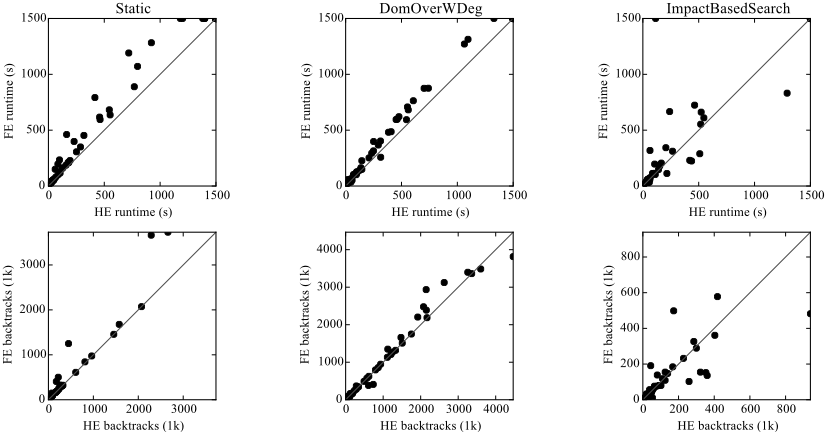

limits to hi the amount of energy spent by a task i at any given time which shifts the energy later on the schedule. The fully-elastic relaxation consumes the bottom part of the resource entirely and packs the remaining energy as soon as possible on the upper part. The horizontally-elastic relaxation might not fully consume the bottom part and does not necessarily pack the remaining energy at the earliest time on the upper part. Consider the instance with C = 3 and five tasks whose parameters hesti↪ lcti↪ pi↪ hii are x : h0↪ 4↪ 2↪ 1i, y : h1↪ 4↪ 1↪ 3i, z : h2↪ 4↪ 1↪ 3i, w : h2↪ 4↪ 1↪ 1i, and v : h1↪ 10↪ 3↪ 1i. We get adjFv = 2 < adjHv = 3 for the precedence ¶x↪ y↪ z↪ w♦ <· v. ⇤

9 Experimental results

We implemented the algorithms for the Choco 2 solver and tried them on the benchmarks BL [Baptiste and Le Pape, 2000] and PSPLib [Kolisch and Sprecher, 1997] of Resource Constrained Project Scheduling Problems (RCPSP). This problem has multiple resources of varied capacities on which the tasks, subject to precedence constraints, are simultaneously executed. We minimize the makespan. The base model has one starting time variable per task, one makespan variable, and one CUMULATIVE constraint per resource for which the Time-Table rule is enforced [Beldiceanu and Carlsson, 2002]. From this common core, we create two models that are compared against each other. In the horizontallyelastic model, we enforce the Overload Check and EdgeFinder rules as explained in the previous sections. In the fully-elastic model, we rather post our implementation of a constraint that enforces the Overload Check and Edge-Finder rules as described by [Vil´ım, 2009]. We used three different branching heuristics: a static variable and value ordering, DomOverWDeg [Boussemart et al., 2004], and Impact Based Search [Refalo, 2004]. All experiments were run on an Intel Xeon X5560 2.667GHz quad-core processor.

Figure 2 compares runtimes and backtracks for both models. We only report instances that were solved within 25 minutes. For the highly-cumulative instances from the BL benchmark, our method gives a speedup for 85%, 82% and 63% of the instances using the static, the DomOverWDeg and the Impact Based Search heuristics. The Impact Based Search leads to the lesser improvement since it tends not to branch on values that would be filtered. For the highly-disjunctive instances from the PSPLib benchmark, we notice a lesser improvement of runtimes since the instances are generally easier to resolve. Our method still allows a speedup for 75% of the instances for all three heuristics.

The horizontally-elastic relaxation grants a significant improvement in the runtimes, although not as significant for the backtracks. This is explained by Vil´ım's algorithm that processes a large number of detected precedences that do not lead to adjustments. We observed that our algorithm only discovers precedences that lead to adjusments. Moreover, our algorithm processes each precedence in linear time.

10 Conclusion

We generalized the Overload Check and Edge-Finder rules using a function of earliest completion time (ect). We introduced a stronger relaxation of ect. We presented an innovative data structure used in two new algorithms that enforce the Overload Check and Edge-Finder rules. Experimental results demonstrate the effectiveness of our method. In fact, our algorithms solved many RCPSP instances with fewer backtracks and in faster times than the state-of-the-art algorithms.