
Decoupled Strong Stubborn Sets
Proceedings of the Twenty-Fifth International Joint Conference on Artificial Intelligence. Pages 3110-3115.
Abstract
Recent work has introduced fork-decoupled search, addressing classical planning problems where a single center component provides preconditions for several leaf components. Given a fixed center path πC, the leaf moves compliant with πC can then be scheduled independently for each leaf. Fork-decoupled search thus searches over center paths only, maintaining the compliant paths for each leaf separately. This can yield dramatic benefits. It is empirically complementary to partial order reduction via strong stubborn sets, in that each method yields its strongest reductions in different benchmarks. Here we show that the two methods can be combined, in the form of strong stubborn sets for fork-decoupled search. This can yield exponential advantages relative to both methods. Empirically, the combination reliably inherits the best of its components, and often outperforms both.
- [Alkhazraji et al., 2012] Yusra Alkhazraji, Martin Wehrle, Robert Mattmüller, and Malte Helmert. A stubborn set al- gorithm for optimal planning. In Luc De Raedt, Christian Bessiere, Didier Dubois, Patrick Doherty, Paolo Frasconi, Fredrik Heintz, and Peter Lucas, editors, Proceedings of the 20th European Conference on Artificial Intelligence (ECAI 2012), pages 891-892. IOS Press, 2012.
- [Amir and Engelhardt, 2003] Eyal Amir and Barbara Engel- hardt. Factored planning. In Georg Gottlob and Toby Walsh, editors, Proceedings of the 18th International Joint Conference on Artificial Intelligence (IJCAI 2003), pages 929-935.
- Morgan Kaufmann, 2003.
- [Bäckström and Nebel, 1995] Christer Bäckström and Bern- hard Nebel. Complexity results for SAS + planning. Com- putational Intelligence, 11(4):625-655, 1995.
- [Brafman and Domshlak, 2003] Ronen I. Brafman and Carmel Domshlak. Structure and complexity in planning with unary operators. Journal of Artificial Intelligence Research, 18:315-349, 2003.
- [Brafman and Domshlak, 2013] Ronen Brafman and Carmel Domshlak. On the complexity of planning for agent teams and its implications for single agent planning. Artificial Intelligence, 198:52-71, 2013.
- [Fabre et al., 2010] Eric Fabre, Loïg Jezequel, Patrik Haslum, and Sylvie Thiébaux. Cost-optimal factored planning: Promises and pitfalls. In Ronen Brafman, Héctor Geffner, Jörg Hoffmann, and Henry Kautz, editors, Proceedings of the Twentieth International Conference on Automated Planning and Scheduling (ICAPS 2010), pages 65-72. AAAI Press, 2010.
- [Gnad and Hoffmann, 2015a] Daniel Gnad and Jörg Hoff- mann. Beating LM-cut with h max (sometimes): Fork- decoupled state space search. In Ronen Brafman, Carmel Domshlak, Patrik Haslum, and Shlomo Zilberstein, edi- tors, Proceedings of the Twenty-Fifth International Con- ference on Automated Planning and Scheduling (ICAPS 2015), pages 88-96. AAAI Press, 2015.
- [Gnad and Hoffmann, 2015b] Daniel Gnad and Jörg Hoff- mann. From fork decoupling to star-topology decoupling. In Proceedings of the Eighth Annual Symposium on Com- binatorial Search (SoCS 2015), pages 53-61. AAAI Press, 2015. Gnad et al., 2016]
- Daniel Gnad, Martin Wehrle, and Jörg Hoffmann. Decoupled strong stubborn sets (technical report). Technical report, Saarland University, 2016. Available at http://fai.cs.uni-saarland.de/hoffmann/papers/ ijcai16a-tr.pdf. Link
- [Helmert and Domshlak, 2009] Malte Helmert and Carmel Domshlak. Landmarks, critical paths and abstractions: What's the difference anyway? In Alfonso Gerevini, Adele Howe, Amedeo Cesta, and Ioannis Refanidis, ed- itors, Proceedings of the Nineteenth International Con- ference on Automated Planning and Scheduling (ICAPS 2009), pages 162-169. AAAI Press, 2009.
- [Helmert, 2006] Malte Helmert. The Fast Downward plan- ning system. Journal of Artificial Intelligence Research, 26:191-246, 2006.
- [Jonsson and Bäckström, 1995] Peter Jonsson and Christer Bäckström. Incremental planning. In Malik Ghallab and Alfredo Milani, editors, New Directions in AI Planning: EWSP '95 -3rd European Workshop on Planning, vol- ume 31 of Frontiers in Artificial Intelligence and Applica- tions, pages 79-90, Amsterdam, 1995. IOS Press.
- [Kelareva et al., 2007] Elena Kelareva, Olivier Buffet, Jinbo Huang, and Sylvie Thiébaux. Factored planning using de- composition trees. In Manuela M. Veloso, editor, Proceed- ings of the 20th International Joint Conference on Artifi- cial Intelligence (IJCAI 2007), pages 1942-1947, 2007. IJCAI
- [Knoblock, 1994] Craig A. Knoblock. Automatically gen- erating abstractions for planning. Artificial Intelligence, 68(2):243-302, 1994.
- [Valmari, 1989] Antti Valmari. Stubborn sets for reduced state space generation. In Grzegorz Rozenberg, editor, Proceedings of the 10th International Conference on Ap- plications and Theory of Petri Nets (APN 1989), volume 483 of Lecture Notes in Computer Science, pages 491- 515. Springer-Verlag, 1989.
- [Wehrle and Helmert, 2012] Martin Wehrle and Malte Helmert. About partial order reduction in planning and computer aided verification. In Lee McCluskey, Brian Williams, José Reinaldo Silva, and Blai Bonet, editors, Proceedings of the Twenty-Second International Con- ference on Automated Planning and Scheduling (ICAPS 2012). AAAI Press, 2012.
- [Wehrle and Helmert, 2014] Martin Wehrle and Malte Helmert. Efficient stubborn sets: Generalized algorithms and selection strategies. In Proceedings of the Twenty- Fourth International Conference on Automated Planning and Scheduling (ICAPS 2014), pages 323-331. AAAI Press, 2014.
References were extracted automatically from the PDF and may contain errors.
Full text extracted automatically from the PDF; figures, tables and equations may differ. The PDF is the version of record.
1 Introduction
In classical AI planning, the task is to find a sequence of actions leading from a given initial state to a state that satisfies a given goal condition, in a large deterministic transition system (the task's state space). Gnad and Hoffmann [2015a] (henceforth: GH) have recently introduced a new approach, fork-decoupled search, to decompose the state space. The approach relates to factored planning (e.g. [Amir and Engelhardt, 2003; Kelareva et al., 2007; Fabre et al., 2010; Brafman and Domshlak, 2013]), where the factors are disjoint subsets of state variables. Fork-decoupled search assumes that the factors induce a fork structure: a single center factor provides preconditions for several leaf factors, and no other cross-factor interactions exist. As GH show, such a fork factoring, if one exists, can be easily identified in a pre-process to planning, based on the task's causal graph (e.g. [Knoblock, 1994; Jonsson and B¨ackstr¨om, 1995; Brafman and Domshlak, 2003; Helmert, 2006]).
In a fork factoring, the leaves are "conditionally independent", in the sense that, given a fixed center path ⇡C , the compliant leaf moves - those leaf moves enabled by the preconditions supplied along ⇡C - can be scheduled independently for each leaf. This can be exploited by searching only over
J ¨org Hoffmann
Saarland University Saarbr¨ucken, Germany hoffmann@cs.uni-saarland.de
center paths, and maintaining the possible compliant paths separately for each leaf, thus avoiding the enumeration of state combinations across leaves. GH show how to employ standard heuristic search planning algorithms, preserving optimality guarantees. They obtain dramatic benefits in several International Planning Competition (IPC) benchmarks.
Fork-decoupling can be thought of as a reformulation of the search space. Can known search reduction methods be applied on the reformulated search space as well? We herein answer this in the affirmative for a prominent reduction method, namely state-of-the-art partial order reduction via strong stubborn sets (SSS) [Valmari, 1989; Alkhazraji et al., 2012; Wehrle and Helmert, 2012; 2014]. This method prunes applicable actions on states s during (standard, nondecoupled) search, namely those not contained in an SSS for s. The SSS is guaranteed to contain at least one action starting an optimal plan for s, so optimality is preserved.
Fork-decoupled search and SSS yield their respective best reductions in different IPC domains. We show that the two methods are indeed exponentially separated, i.e., that there are cases where one yields exponentially stronger reductions than the other. We show how to combine them in the form of decoupled strong stubborn sets (DSSS), for fork-decoupled search. We show that this combination is exponentially separated from both its components. There are cases - not complex artificial examples, but simple variants of the Logistics benchmark - where DSSS yield exponentially stronger reductions than both fork-decoupling and SSS. Empirically, DSSS reliably inherit the strengths of each component, and sometimes outperform both. In some cases, DSSS even is "more than the sum of its components", yielding a stronger reduction in fork-decoupled search than SSS do in standard search.
For space reasons, we give proof sketches only. The full proofs are available in an online TR [Gnad et al., 2016].
2 Background
We employ a finite-domain state variable formalization of planning (e.g. [B¨ackstr¨om and Nebel, 1995; Helmert, 2006]). A finite-domain representation planning task, short FDR task, is a tuple ⇧ = hV↪A↪ s0↪ s?i. V is a set of state variables, each v 2 V associated with a finite domain D(v). We identify (partial) variable assignments with sets of variable/value pairs. A complete assignment to V is a state. s0 is the initial state, and the goal s? is a partial assignment to V . A
is a finite set of actions. Each action a 2 A is a triple hpre(a)↪ e↵ (a)↪ cost(a)i where the precondition pre(a) and effect e↵ (a) are partial assignments to V, with e↵ (a) 6= ;; cost(a) 2 R0+ is a's non-negative cost.
Given a partial assignment p, by vars(p) ✓ V we denote the subset of state variables on which p is defined. For V ✓ vars(p), by p[V ] we denote the assignment to V made by p. Action a is applicable in state s if s ♣= pre(a), i.e., pre(a) ✓ s. Applying a in s changes the value of v 2 vars(e↵ (a)) to e↵ (a)[v], and leaves s unchanged elsewhere. A plan for ⇧ is an action sequence ⇡ applicable in s0 and ending in a state s such that s ♣= s?. The plan is optimal if its summed-up cost, denoted cost(⇡), is minimal among all plans for ⇧.
We next give a summary of fork-decoupled search. We will often write "decoupled" instead of "fork-decoupled".
A factoring F is a partition of V. F is a fork factoring if ♣F♣ ≥ 2 and there exists F C 2 F s.t. the arcs in F's interaction graph are exactly ¶(F C ↪ F L) ♣ F L 2 F ∩¶F C ♦♦. Here, the interaction graph is the quotient of the task's causal graph over F, i.e., it contains an arc (F↪ F 0 ) if there exists a 2 A s.t. F \ [vars(pre(a)) [ vars(e↵ (a))] 6= ; and F 0 \ vars(e↵ (a)) 6= ;. We refer to F C as the center of F, and to all other factors F L 2 F L := F ∩ ¶F C ♦ as its leaves.
Not every task ⇧ has a fork factoring. We assume GH's approach of analyzing ⇧'s causal graph in a pre-process, identifying a fork factoring if one exists, else abstaining from solving ⇧. In what follows, assume a fork factoring F.
As a running example, consider a Logistics-style planning task with 1 truck variable t, N package variables pi, and two locations A and B. The truck and all packages are initially at A, and the goal is for the packages to be at B. The actions (unit costs) are drive, load, and unload, with the usual preconditions and effects (e.g. load(t↪ pi↪A) requires both t and pi to be at A, and moves pi into the truck). Setting ¶t♦ as the center and each ¶pi♦ as a leaf, we obtain a fork factoring.
Given the structure of the interaction graph, every action affects (touches in its effect) either only F C , or only one leaf F L. We refer to the former kind as center actions, and to the latter kind as leaf actions. Observe that center actions do not have any preconditions on leaves. Furthermore, if leaf action a affects leaf F L, then it can be preconditioned only on F C and F L, i.e., vars(pre(a)) ✓ F C [ F L.
Due to these action behaviors, a fork factoring encapsulates a particular form of "conditional independence" between leaves. Assume a center path ⇡C , i.e., a sequence of center actions applicable to s0. A leaf path is a sequence of leaf actions applicable to s0 when ignoring preconditions on F C . A leaf path ⇡L complies with ⇡C if it uses only the center preconditions supplied along ⇡C , i.e., if ⇡L can be scheduled alongside ⇡C so that the combined action sequence is applicable in s0. Intuitively, fixing ⇡C , the compliant leaf paths are the possible leaf moves given ⇡C . Observe that these possible moves are independent across leaf factors F L, i.e., for each F L we can choose a compliant ⇡L independently from that choice for any other leaf factor. Hence we can search over center paths ⇡C only, maintaining all possible compliant paths separately for each leaf. We commit to the actual choices of compliant leaf paths only when the goal is reached.
Concretely, a decoupled state sF is given by a center path
⇡C (sF ). It is associated with its center state ct(sF ), simply the outcome of applying ⇡C (sF ) to s0[F C ]; and with its pricing function prices(sF ). The latter maps each leaf state sL, i.e., each value assignment to some leaf F L, to its price, defined as the cost of a cheapest leaf path that complies with ⇡C (sF ) and ends in sL (or 1 if no such path exists). Pricing functions can be maintained in time low-order polynomial in the size of the individual F L state spaces; we omit the details for space reasons. Note the word "price": prices(sF )[sL] is not a cost we have already paid; rather, it is the cost we will have to pay in case we commit to sL in sF later on.
The initial decoupled state sF0 results from the empty center path ⇡C (sF0 ) = hi. We denote by ReachedL(sF ) the set of leaf states sL reachable in sF , i.e., where prices(sF )[sL] < 1. A goal decoupled state sF? is one with a goal center state ct(sF? ) ♣= s?[F C ] and where, for every leaf factor F L 2 F L, there exists a reachable goal leaf state sL, i.e., sL 2 ReachedL(sF? ) such that sL ♣= s?[F L]. The actions applicable in sF are those center actions whose precondition is satisfied in ct(sF ) (recall here that we do not branch over leaf actions). Applying a to sF results in tF where ⇡C (tF ) := ⇡C (sF ) ◦ hai, and ct(tF ) as well as prices(tF ) arise from ⇡C (tF ) as defined above.
In our example, ct(sF0 ) = ¶(t↪A)♦, and for each pi the price of (pi↪A) is 0, that of (pi↪ t) is 1, and that of (pi↪B) is 1. Observe here that the prices represent possible package moves given the initial center state, rather than moves we have already committed to. The only action applicable to sF0 in the decoupled search is the center action drive(t↪A↪B), leading to the goal decoupled state sF? where ct(sF? ) = ¶(t↪B)♦ and the prices are as before except that (pi↪ B) now has price 2, i.e., the package goals are reachable.
Once a goal decoupled state sF? is reached, a plan ⇡ for the input task ⇧ can be constructed by augmenting the center path ⇡C (sF? ) with compliant leaf paths ending in goal leaf states sL? (i.e., we now select such leaf paths, and commit to them). In our example, for each pi we may select the compliant leaf path hload(t↪ pi↪ A)↪unload(t↪ pi↪ B)i.
LocalCost(sF? ) is optimal for sF? (locally optimal) but not necessarily optimal for ⇧ (globally optimal). Indeed, it can happen that, from sF? , a better plan can be obtained from a descendant of sF? . This is because, with additional center actions, cheaper leaf paths may become available. For example, say in sF the leaf goal have-car has price 1000 via the applicable leaf action buy-car. But if we apply a center action getmanager-job, then the leaf action get-company-car becomes applicable, reducing the leaf goal price to 0.
Selecting, for the plan ⇡, the cheapest compliant paths ending in the goal leaf states sL? , by construction we have cost(⇡) = cost(⇡C (sF? )) + PF L2F L prices(sF? )[sL? ]. If we select sL? with minimal prices(sF? )[sL? ], such ⇡ is optimal among the plans for ⇧ whose center action subsequence is ⇡C (sF? ). Given this, we refer to the cost of such ⇡ as the local cost of sF? , denoted LocalCost(sF? ). We set LocalCost(sF ) :=1 for non-goal decoupled states sF .
In contrast to the standard setting, to guarantee optimality one must therefore continue the search on goal decoupled states (GH show that standard search algorithms are easy to adapt to this situation). The purpose of such search, trying to decrease leaf prices, differs from that of non-goal decoupled states, trying to reach the goal in the first place. Our design of strong stubborn sets for decoupled search distinguishes between the two cases.
3 SSS for Non-Goal Decoupled States
We show that, for non-goal decoupled states, the definition of strong stubborn sets (SSS) for planning [Alkhazraji et al., 2012] can be extended to decoupled search by suitable extensions of its basic components.
A SSS for a given state s is a set Ts ✓ A constructed so that, for every plan ⇡ for s, at least one permutation of ⇡ starts with an action a 2 Ts. Hence SSS are fundamentally based on the concept of "plans for a given state". That concept is trivial for classical state spaces. But in decoupled state spaces the structure of "states" sF is more complex. GH did not require, so did not introduce, such a concept. For our purposes, the following notions will suffice.
A path ⇡F in the decoupled state space is a decoupled plan for sF if it leads from sF to a goal decoupled state. We say that sF is solvable if at least one such ⇡F exists. We denote the center-action sequence underlying ⇡F by ⇡C (⇡F ). The completion plan given ⇡F , denoted ComPlan(⇡F ), consists of ⇡C (⇡F ) together with cheapest goal leaf paths ⇡L compliant with ⇡C (sF ) ◦ ⇡C (⇡F ), ending in cheapest goal leaf states. In other words, ComPlan(⇡F ) collects the postfix path for the center, and the complete path for each leaf. Observe that ComPlan(⇡F ) is not uniquely defined, as there may be multiple suitable ⇡L. For our purposes, this does not matter and we assume any suitable choice of ⇡L. We say that ⇡F is optimal if cost(ComPlan(⇡F )) is minimal among all decoupled plans for sF . In our running example, assume a third location C and the road map A ! B ! C. Say we apply drive(t↪A↪B) to sF0 to obtain sF . Then ⇡C := hdrive(t↪B↪C)i yields a decoupled plan ⇡F for sF , and ComPlan(⇡F ) consists of all load(t↪ pi↪ A) actions, then ⇡C , then all unload(t↪ pi↪ C) actions.
Clearly, to preserve optimality, it suffices for Ts to contain at least one center action starting an optimal decoupled plan for sF . Towards identifying sets Ts qualifying for this, we will need to focus exclusively on the part of the completion plan "behind" sF . We denote this by PostPlan(⇡F ), the postfix plan. The center action subsequence in PostPlan(⇡F ) is ⇡C (⇡F ). For any leaf factor F L, say ⇡L = haL1 ↪ ▷ ▷ ▷ ↪ aLn i is the goal leaf path for F L in ComPlan(⇡F ), traversing leaf states hsL0 ↪ ▷ ▷ ▷ ↪ sLn i. Then the leaf action subsequence for F L in PostPlan(⇡C ) is defined as haLi+1 ↪ ▷ ▷ ▷ ↪ aLn i, where i is the highest index for which sLi 2 ReachedL(sF ). In other words, we consider the postfix of ⇡L not contained in ReachedL(sF ).
Two notions, of completion plan and postfix plan, are required because postfix plans are (in contrast to the standard setting) not suited to define optimality. The decoupled plan leading to the cheapest postfix plan may differ from that leading to the cheapest completion plan. This is because the postfix plan ignores the price of the sF leaf states it starts from.
The original definition of SSS in states s relies on the basic concepts of disjunctive action landmarks, action interference, necessary enabling sets, and action applicability. For a corresponding definition for decoupled states sF , the concept of action interference remains the same, but all other concepts must be extended. We start with applicability:
Definition 1 (Action Applicability). Let sF be a decoupled state. A center action a is applicable in sF if ct(sF ) ♣= pre(a). A leaf action a affecting leaf F L is applicable in sF if ct(sF ) ♣= pre(a)[F C ], and there exists a leaf state sL 2 ReachedL(sF ) such that sL ♣= pre(a)[F L]. The set of actions applicable in sF is denoted with app dec (sF ).
Note that this definition encompasses both, center actions and leaf actions. This is in contrast to the decoupled search which branches only over (applicable) center actions. Thus the notion of "applicability" as per Definition 1 is different from the notion used in decoupled search. It is better suited for the definition of strong stubborn sets, lending itself to a direct extension of the original definition.
Let us next focus on the concept of necessary enabling sets. Given an action a whose preconditions are not true, a necessary enabling set should be a set of actions one of which must necessarily be applied in order to enable a. In the standard setting, such a set is trivial to obtain, by picking a precondition value not currently true and selecting all actions achieving that value. In decoupled search, this is not as easy because decoupled states do not assign unique values to leaf-factor state variables. We adjust the concept as follows:
Definition 2 (Decoupled Necessary Enabling Set). Let sF be a decoupled state, and let a be an inapplicable action a 62 app dec (sF ). An action set A is a decoupled necessary enabling set for a in sF if either of the following cases holds:
- (i) A = ¶a0 2 A ♣ e↵ (a0 )[v] = pre(a)[v]♦ where v 2 vars(pre(a)) \ F C s.t. ct(sF )[v] 6= pre(a)[v].
- (iii) A = Sv2V ¶a0 2 A ♣ e↵ (a0 )[v] = pre(a)[v]♦ where V 6= ; is the set of all v 2 vars(pre(a)) s.t. exists sL 2 ReachedL(sF ) with sL 6♣= pre(a)[v].
- (ii) A = ¶a0 2 A ♣ e↵ (a0 )[v] = pre(a)[v]♦ where v 2 vars(pre(a)) ∩F C s.t., for all sL 2 ReachedL(sF ), we have sL 6♣= pre(a)[v].
Case (i) in this definition corresponds to the standard setting, where A are the achievers of an open precondition on the center, whose assignment is fixed in sF . Case (ii) captures the situation where a leaf precondition is false in all reachable leaf states. Case (iii) is relevant because a leaf action may have several preconditions, each satisfied by some reachable leaf state, but not all satisfied jointly in any reachable leaf state. We then collect the achievers of preconditions open in any reachable leaf state. Clearly, in every case at least one a0 2 A must be used by any postfix plan for sF that contains a. At least one of the cases must apply as a 62 app dec (sF ). For center actions, only case (i) is possible. For leaf actions, we first test (ii), then (iii), and finally (i), the motivation being to focus on the open center preconditions "closest" to sF .
We finally need to adjust the concept of disjunctive action landmarks. Given our notion of postfix plans, this is direct:
Definition 3 (Decoupled Disjunctive Action Landmark). Let sF be a non-goal decoupled state. An action set L is a decoupled disjunctive action landmark for sF if, for all decoupled plans ⇡C for sF , we have PostPlan(⇡C ) \ L 6= ;.
In our implementation, we find decoupled disjunctive action landmarks simply in terms of a necessary enabling set for the goal condition s?, i.e., exactly as in Definition 2 but using s? as the precondition of a hypothetical action a.
The last basic concept we need is the standard notion of interference between pairs of actions. We say that a and a0 interfere if ex. v s.t. e↵ (a0 )[v] 6= e↵ (a)[v] or e↵ (a)[v] 6= pre(a0 )[v] or e↵ (a0 )[v] 6= pre(a)[v]. Decoupled strong stubborn sets are now defined as follows:
Definition 4 (DSSS for Non-Goal Decoupled States). Let sF be a non-goal decoupled state. An action set Ts is a decoupled strong stubborn set (DSSS) for sF if the following conditions hold:
- (i) Ts contains a decoupled disjunctive action landmark.
- (ii) For all actions a 2 Ts and a ◁2 app dec (sF ), Ts contains a decoupled necessary enabling set for a.
- (iii) For all center actions a 2 Ts and a 2 app dec (sF ), Ts contains all actions that interfere with a.
Thanks to the adapted basic concepts, this definition mirrors the original one [Alkhazraji et al., 2012]. Intuitively, condition (i) ensures that Ts makes progress to the goal; condition (ii) ensures that Ts backchains all the way to the current state; condition (iii) ensures that, if we branch over a, then we also branch over all actions that may be in conflict with a. All three conditions are identical to the respective original one, modulo the adapted basic concepts. The single exception is the restriction to center actions in condition (iii). We do not need to include interfering actions for applicable leaf actions. That is so because postfix plans do not contain applicable leaf actions anyhow: everything that can be done using such actions is already reachable in sF .
By adapting the proof arguments from the standard setting, one can show that DSSS preserve optimality:
Theorem 1. Let sF be a solvable non-goal decoupled state. Let Ts be a DSSS in sF . Then Ts contains a center action that starts an optimal decoupled plan for sF .
The proof considers any decoupled plan ⇡F for sF . Denote ⇡ = ha1↪ ▷ ▷ ▷ ↪ ami = PostPlan(⇡F ), and let i be the smallest index so that ai 2 Ts. For the same reasons as shown in the original proof for SSS [Alkhazraji et al., 2012], such ai exists, must be applicable, and - together with the fact that ai must be a center action, as PostPlan(sF ) does not contain any applicable leaf actions - can be moved to the front of ⇡.
4 SSS for Goal Decoupled States
Say we are facing a goal decoupled state sF? . Instead of actions required for reaching the goal, we need to capture actions required to reduce the leaf-goal prices. One may consider to define landmarks relative to the decoupled plans reaching states tF? where LocalCost(tF? ) < LocalCost(sF? ), and then re-use the remainder of Definition 4 unchanged. Indeed, this was our first solution attempt. The problem is that the landmark actions may pertain to leaf states already reached, only at non-optimal prices; and then we may miss the actions required to reduce those prices.
To illustrate, say that, as before, we have a leaf action buy-car (cost 1000) applicable to sF , and a center action get-manager-job which enables leaf action get-company-car (cost 0). However, now the leaf goal is not have-car, but be-at-NYC for which another leaf action drive-car is needed. Then ¶drive-car♦ is a landmark: Any optimal completion plan for sF has to use this action behind sF , i.e., after applying another center action. But drive-car is applicable in sF , so Definition 4 would stop here, and Ts would not contain get-company-car. In other words, the notion of necessary enabling sets is suited to reachability but is not suited to capture what's needed to decrease prices.
We tackle this situation through a notion of frontier actions, required to make any progress on the prices:
Definition 5 (Frontier Action). Let sF? be a decoupled goal state, and let a be a leaf action affecting leaf F L. We say that a is a frontier action in sF? if (i) a 62 app dec (sF? ); and (ii) there exists a leaf state sL 2 ReachedL(sF? ) such that sL ♣= pre(a)[F L], and, denoting the outcome of applying a to sL with tL, prices(sF? )[sL] + cost(a) < prices(sF? )[tL]. The frontier of sF? is the set of all frontier actions in sF? .
In words, the frontier consists of those leaf actions that are not currently applicable, but enabling whose center precondition would result in a reduced price for at least one leaf state. This set of actions now takes the role of the landmark:
Definition 6 (DSSS for Goal Decoupled States). Let sF? be a goal decoupled state. An action set Ts is a decoupled strong stubborn set (DSSS) for sF? if the following conditions hold:
- (i) Ts contains the frontier of sF? .
- (ii) For all actions a 2 Ts and a ◁2 app dec (sF? ), Ts contains a decoupled necessary enabling set for a.
- (iii) For all center actions a 2 Ts and a 2 app dec (sF? ), Ts contains all actions that interfere with a.
Consider now a state sF? where hi is not an optimal decoupled plan, i.e., we can find a better plan below sF? . Consider any decoupled plan ⇡F leading to tF? where LocalCost(tF? ) < LocalCost(sF? ). Then ComPlan(⇡F ) contains at least one frontier action aF , intuitively because these actions are needed to decrease prices relative to sF? . By construction, aF has a center precondition not satisfied in sF? . Therefore, with the inclusion of necessary enabling sets, we get that Ts must contain an applicable center action a of ⇡F . For the same reasons as before we can move a to the front, proving that DSSS as per Definition 6 preserve optimality:
Theorem 2. Let sF? be a goal decoupled state for which hi is not an optimal decoupled plan. Let Ts be a decoupled strong stubborn set for sF? . Then Ts contains a center action that starts an optimal decoupled plan for sF? .
Observe that Frontier(sF ) may be empty. In that case, the DSSS will be empty, too. This is valid because, in this case, necessarily hi is an optimal decoupled plan for sF? , i.e., no better plan can be found below sF? and the search can stop.
5 Exponential Separations
Before proceeding to the empirical part of our research, let us state some basic theoretical facts evaluating the power of DSSS. We say that a search space reduction method X is exponentially separated from a method Y if there exists a parameterized example family F such that, on F, X yields an exponentially stronger reduction than Y.
Decoupled search and SSS are complementary in that each is exponentially separated from the other:
Theorem 3. Fork-decoupled search is exponentially separated from SSS, and vice versa.
Our running example with locations A and B is a suitable family F for the first claim. There are only 3 reachable decoupled states (sF0 ; drive to B; drive back). But SSS do not yield any pruning because, in any state s, to make progress to the goal, Ts must include an applicable (un)load action; which interferes with the applicable drive action; which in turn interferes with all applicable (un)load actions. The opposite claim follows from examples, e.g. IPC Parcprinter, with no fork factoring but strong SSS pruning.
Trivially, DSSS is exponentially separated from each of fork-decoupled search and SSS, simply because DSSS naturally generalizes each of these components, so we can use the same families F as in Theorem 3. As a much stronger testimony to the power of DSSS, there are cases where it is exponentially separated from both its components:
Theorem 4. There exists a parameterized example family F such that, on F, DSSS yields an exponentially stronger reduction than both, fork-decoupled search and SSS.
Two suitable families F arise from simple modifications of our running example. First, say we have M trucks and N ⇤M packages, where each truck ti is associated with a group of N packages that only ti can transport. The number of reachable decoupled states is exponential in M because all trucks must be in the center factor. The SSS-pruned reachable standard state space has size exponential in N because including an (un)load action into Ts necessitates, due to interference via the truck move as above, to include all applicable (un)load actions for the respective package group. However, in decoupled search with DSSS pruning, there are only M reachable states. This is because the two sources of pruning power combine gracefully. Decoupling gets rid of the blow-up in N (the packages within a group become independent leaves), while DSSS gets rid of the blow-up in M (only a single truck is committed to at a time).
In our second example, DSSS even is exponentially more than the sum of its components: stubborn sets have exponentially more impact on the decoupled search space than on the standard one. Say we have N packages and M trucks (where every truck may transport every package). Then decoupled search blows up in M, and SSS does not do anything because any package may require any truck. Applying DSSS to decoupled search, no truck move is pruned in sF0 . However, after applying any one drive(ti↪A↪B) action, all package prices are the cheapest possible ones, the frontier is empty, and DSSS stops the search. So, again, there are only M reachable states. As we shall see next, similar phenomena seem to occur in the standard IPC Logistics benchmarks.
6 Experiments
We extended GH's implementation of fork-decoupled search in FD [Helmert, 2006]. To extract the fork factorings, we use GH's method. It computes the strongly connected components (SCCs) of the causal graph, and, arranging the acyclic graph of SCCs with roots "at the top" and leaves "at the bottom", greedily finds a "horizontal line" through that graph. The part above the line becomes the center, each weakly connected component below the line becomes a leaf. The technique abstains if there is 1 leaf, the rationale being that decoupling pays off mainly through avoiding enumeration across > 1 leaves. We show results for those benchmarks on which the technique does not abstain. From the International Planning Competition (IPC) STRIPS benchmarks ('98-'14), this is the case for instances from 12 domains.
We focus here on optimal planning, the main purpose of the optimality-preserving pruning via strong stubborn sets. We run A⇤ with a blind heuristic as a measure of search space size, and with LM-cut [Helmert and Domshlak, 2009] as a representative of the state of the art, using GH's method (Fork-Decoupled A⇤ ) to adopt these techniques for decoupled search. We compare decoupled search with DSSS pruning (simply referred to as "DSSS" in what follows) against decoupled search without that pruning ("DS" in what follows). We furthermore compare against A⇤ in the standard state space without pruning ("A⇤ " in what follows), and with SSS pruning ("SSS" in what follows). All experiments are run on a cluster of Intel E5-2660 machines running at 2.20 GHz, with time (memory) cut-offs of 30 minutes (4 GB).
| Blind Heuristic | LM-cut | ||||||||
|---|---|---|---|---|---|---|---|---|---|
| Domain | # | A⇤ | SSS | DS | DSSS | A⇤ | SSS | DS | DSSS |
| Driverlog | 20 | 7 | 7 | 11 | 11 | 13 | 13 | 13 | 13 |
| Logistics'00 | 28 | 10 | 10 | 22 | 24 | 20 | 20 | 28 | 28 |
| Logistics'98 | 35 | 2 | 2 | 4 | 5 | 6 | 6 | 6 | 6 |
| Miconic | 145 | 50 | 45 | 35 | 36 | 136 | 136 | 135 | 135 |
| NoMystery | 20 | 8 | 7 | 17 | 15 | 14 | 14 | 20 | 19 |
| Pathways | 29 | 3 | 3 | 3 | 3 | 4 | 4 | 4 | 4 |
| Rovers | 40 | 6 | 7 | 7 | 9 | 7 | 9 | 9 | 11 |
| Satellite | 36 | 6 | 6 | 6 | 6 | 7 | 11 | 7 | 11 |
| TPP | 27 | 5 | 5 | 23 | 22 | 5 | 5 | 18 | 18 |
| Wood'08 | 13 | 4 | 6 | 5 | 7 | 6 | 11 | 10 | 11 |
| Wood'11 | 5 | 0 | 1 | 1 | 2 | 2 | 5 | 4 | 5 |
| Zenotravel | 20 | 8 | 7 | 11 | 11 | 13 | 13 | 13 | 13 |
| 418 | 109 | 106 | 145 | 151 | 233 | 247 | 267 | 274 | |
P
Table 1 shows coverage results. The most important comparison for our purposes here is that between DSSS vs. DS, i.e., the direct benefit our pruning technique yields over the baseline search. DSSS is rarely worse (NoMystery -2 and TPP -1 for blind search, only NoMystery -1 for LM-cut). It is often better (6 domains for blind, 4 domains for LMcut), and consequently is better, though not dramatically better, in the overall. Comparing to A⇤ and SSS, we see that DSSS improves DS whenever (i.e., in all domains where) SSS improves A⇤ . Whenever SSS outperforms DS, DSSS fully makes up for this advantage: the per-domain coverage of DSSS dominates that of SSS. The single exception to the latter is Miconic, where DSSS just inherits the weakness (runtime overhead at not much search gain) of decoupled search.
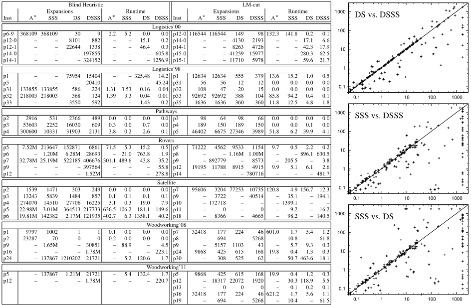
Figure 1 shows fine-grained performance data. Consider first the scatter plots. The plot at the top reveals that DSSS often improves over DS, up to 2 orders of magnitude on commonly solved instances, while bad cases are consistently limited to a moderate overhead. The plot SSS vs. DS shows that, without pruning, decoupled search is in the advantage yet also incurs several bad cases. We see in the plot SSS vs. DSSS that, with DSSS pruning, this risk mostly disappears.
The table in Figure 1 shows data for those domains where DSSS sometimes reduces expansions relative to DS (we discuss the other domains below). For each of blind search and LM-cut, from the instances solved by at least one method, we selected at most 5, namely the most challenging ones (largest expansions under standard A⇤ ). Where these did not include an instance solved by all methods, to exemplify the crosscomparison we included the most challenging such instance.
As the table shows, on those domains where DSSS does yield pruning, it consistently improves over DS, both in expansions and runtime, for both blind search and LM-cut. The behavior in Logistics is especially remarkable. On the standard state space, SSS yields little or no reduction, while in the decoupled state space, DSSS yields strong reductions. This establishes a practical case of DSSS being more than the sum of its components. Compared to SSS, decoupled search with DSSS is superior in Logistics, Pathways, and Rovers, and is inferior in Satellite; the picture in Woodworking is mixed.
On the domains where DSSS does not reduce expansions (Driverlog, Miconic, NoMystery, TPP, and Zenotravel), a runtime overhead is incurred. For blind search, we get slowdown factors up to 218▷5 in NoMystery, 26▷9 in TPP, and 4▷8 in the other 3 domains. This is due to the small perstate search effort in blind search, relative to which computing a DSSS can consume substantial runtime. For the state-of-the-art search using LM-cut, where per-state effort is much higher, the overhead is small. The maximum (geometric mean) slow-down factor is 1▷3 (1▷1) for Driverlog, 2▷0 (1▷0) for Miconic, 3▷1 (2▷2) for NoMystery, 2▷0 (1▷3) for TPP, and 2▷0 (1▷1) for Zenotravel. Using a simple "safety belt" which switches DSSS off after 1000 expansions if no action was pruned, the slow-down disappears in almost all cases.
7 Conclusion
We have shown that fork-decoupled search and strong stubborn sets combine gracefully in theory, and that the combination can yield good results in practice. Our next step will be to extend decoupled strong stubborn sets to star-topology decoupling as per Gnad and Hoffmann [2015b]. More generally, decoupled search is a new paradigm that, presumably, can be fruitfully combined not only with (heuristic search and) strong stubborn sets, but also with other search techniques like symmetry reduction or symbolic representations.
Acknowledgments
Daniel Gnad was partially supported by the German Research Foundation (DFG), as part of project grant HO 2169/61, "Star-Topology Decoupled State Space Search". Martin Wehrle was supported by the Swiss National Science Foundation (SNSF) as part of the project "Automated Reformulation and Pruning in Factored State Spaces (ARAP)".
@inproceedings{ijcai2016p441,
  title     = {Decoupled Strong Stubborn Sets},
  author    = {Gnad, Daniel and Wehrle, Martin and Hoffmann, Jörg},
  booktitle = {Proceedings of the Twenty-Fifth International Joint Conference on
               Artificial Intelligence, {IJCAI-16}},
  publisher = {AAAI Press / International Joint Conferences on Artificial Intelligence},
  editor    = {Subbarao Kambhampati},
  pages     = {3110--3115},
  year      = {2016},
  month     = {7},
  url       = {https://ijcai.org/proceedings/2016/441},
}
TY - CPAPER TI - Decoupled Strong Stubborn Sets AU - Gnad, Daniel AU - Wehrle, Martin AU - Hoffmann, Jörg T2 - Proceedings of the Twenty-Fifth International Joint Conference on Artificial Intelligence, IJCAI-16 PB - AAAI Press / International Joint Conferences on Artificial Intelligence PY - 2016 SP - 3110 EP - 3115 UR - https://ijcai.org/proceedings/2016/441 ER -Copied
Machine-readable versions of this paper, for tools and AI agents:





