Hierarchical Model Predictive Control for Multi-Robot Navigation

1 Introduction

The navigation of multi-robot systems is the problem of how to control a group of robots making them move from starting states to their goal states. It has recently attracted increasing attention in the robotics and multi-agent fields. Most of existing work has been devoted to control problems in which a reference trajectory is given as a known condition [Rosales et al., 2011; Antonelli et al., 2013; Tian and Sarkar, 2012]. Given the reference trajectory, the techniques aim to drive a group of robots to cooperatively move toward a destination with a desired formation. Since the predefined reference trajectory can act as explicit landmarks to guide the robots in the navigation, convergence of the methods, referred as stability, and the collision avoidance, referred as feasibility, are naturally guaranteed.

We consider the case where no reference trajectory is available in advance. The situation occurs in many practical applications, particularly when the knowledge of a navigation environment cannot be sufficiently obtained. Undoubtedly, ensuring the stability is the most important requirement of the method for no reference trajectory navigation. Heuristic-search based methods are quite popular in this area [Calliess et al., 2014; Godoy et al., 2015; Janovsky et al., 2014]. However, most of them are unable to provide theoretical results aiding in guaranteeing the stability and feasibility. They may produce trajectories that cause robots to stick at one point or never converge to the target position. That is why a failure ratio becomes a primary index when different methods are compared.

⇤Corresponding author: chenxin@nju.edu.cn

Model Predictive Control (MPC) is one of the most popular optimal control techniques that derives the current control action of a system from its explicit model with constraints and its current state. For centralized MPC (CMPC), the theory of feasibility and stability has been adequately studied [Mayne et al., 2000; Olfati-Saber et al., 2003; Dunbar and Murray, 2002]. However, as CMPC composes together the cost function, the constraints and the dynamics of every robot into a big optimal problem and relies on a central controller to solve the input actions for all robots, it is prone to be computationally prohibitive.

An intuitive method for solving the computational issue is to decompose the big problem into many independent subproblems, distribute them to many robots and solve it in parallel. In basic distributed MPC (BDMPC) [Keviczky et al., 2004b], each robot's local controller only cares for its neighbours and computes its own actions based on the local knowledge of its neighbours. Such a decomposition simply drops many constraints, thus in theory, it gives no guarantee on feasibility and stability. Sequential distributed MPC (SDMPC) [Kuwata and How, 2011] forces local controllers to make computation according to a pre-defined order. Iterative distributed MPC (IDMPC) [Mercang¨oz and Doyle III, 2007] introduces an iterative computation process to determine the input where each local controller uses MPC to predict its future behavior based on the predicted behaviors of its neighbours received in the last iteration and exchanges it with its neighbours. The process repeats until the solution of the original problem is found. Under certain conditions 1 , SDMPC and IDMPC can ensure stability and feasibility, but at the cost of much more computational time.

The parallel decomposition of the navigation problem continues to be a challenging issue since a successful decomposition must carefully decouple all couplings in the objective functions, constraints and dynamics. It should save the computation time while ensuring stability and feasibility. In this paper we propose a hierarchical MPC (HMPC) scheme to deal with the navigation problem of linear dynamical multirobot systems with no reference trajectory. Different from existing works, our HMPC employs a notion of reachable sets to help with the decomposition. It ensures stability and feasibility while greatly reducing the computation time. It can also deal with problems with nonlinear objective functions, compared to the most recent work based on the Dantzig-Wolfe decomposition [Bourdais et al., 2014] where their objective functions (and constraints) have to be linear.

1 One such condition is that there are only convex constraints involved and the neighbourhood topology for each robot remains unchanged during the whole moving. However, the navigation problem studied in the paper does not meet such a condition.

In the proposed HMPC, each local controller computes its reachable set based on its dynamics and its current state, and then reports it to the central controller. The central controller combines the collected reachable sets with the objective function and the constraints to form an optimization problemwhose solution consists of the target states for every robot. Then, each robot's local controller computes its input according to the target assigned to it. Our reachable set is parameterized with the robot's current state and can be derived off-line. Compared with CMPC, the central controller in HMPC needs to solve a much smaller problem as all variables, that are irrelevant to the objective function, global and local constraints and to all the dynamics, are all shielded by the reachable set. The computation of inputs for each robot also gets an acceleration as they are performed in parallel. In addition, the stability and feasibility of the HMPC can be proved in the same way as the conventional CMPC. In this context, this paper makes the following contributions:

• ÷ We propose a new control scheme HMPC to address the navigation problem without a reference trajectory based on a new efficient decoupling method via reachable sets.
• ÷ We prove the feasibility and stability of the HMPC scheme.
• ÷ We illustrate the performance for HMPC in several navigation scenarios and demonstrate its advantages in comparison to multiple MPC schemes.

2 ProblemFormulation

We consider a multi-robot system S containing N robots on a plane. The behavior of each robot is represented as a discretetime control sub-system and these sub-systems may differ in the dynamic and sampling cycle. Given that the sampling interval of the i-th robot is Ti, the interval of synchronization of all the subsystems is the least common multiple of their sampling intervals. We refer to the interval of synchronization as one collaboration cycle. For the i-th robot, the collaboration cycle is Ki times its local control cycle.

A state of the i-th robot is denoted as qi = [xi↪ yi↪ ˙xi↪ ˙yi]T , where qi↪pos = [xi↪ yi]T and qi↪vel = [ ˙xi↪ ˙yi]T denote the position and velocity along the x-axis and the y-axis, respectively. The dynamic model of the i-th robot is described as the linear discrete-time time-invariant state equality below.

where k denotes the k-th collaboration instant, ki2¶0↪ 1↪ ▷▷▷↪Ki-1♦ represents the ki-th local control instant of the i-th robot, and ui denotes the input. Equation (1b) defines the beginning state of one collaboration cycle as the ending state of the last collaboration cycle. For convenience, we may use qi(k) and ui(k) to represent qi(k↪ 0) and ui(k↪ 0) respectively. Let a convex polytope Ui denote the feasible set of input for the i-th robot:

The input sequence of the i-th robot in the k-th collaboration cycle is denoted by ˜ui(k) , ui(k)↪ ui(k↪ 1)↪ ▷▷▷↪ ui(k↪ Ki-1). The constraint set of the sequence ˜ui(k) is denoted as ˜ Ui:

For a multi-robot system S, let q(k) , [q1(k)↪ ▷▷▷↪ qN(k)] denote the global state of S at the k-th collaboration instant, ˜u(k) , ˜u1(k)↪ ▷▷▷↪ ˜uN(k) denote the (list of) input sequence of S in the k-th collaboration cycle.

In order to avoid collision during the navigation, we define the collision avoidance specification requiring that the (infinity norm) distance between any two robots must not be less than a given safety distance dsafe:

where

The infinite norm of a vector x = [x1↪ ▷▷▷↪ xn]T is defined as kxk1 , max (♣x1♣↪ ▷▷▷↪ ♣xn♣).

Following [Gondhalekar et al., 2009], we define two core concepts for MPC, namely feasibility and stability.

Definition 1. (Feasibility) A MPC controller is recursively feasible iff for any feasible initial state, the actual state ¶q(t)↪ t≥0♦ computed by the controller at every collaboration instant satisfies the collision avoidance specification h(q(t))0.

The definition requires the collision avoidance specification to be met at every control instant, as mentioned in [Gondhalekar et al., 2009]. This definition of feasibility is sufficient to assure that the trajectory satisfies the collision avoidance specification everywhere, if the density of the collaboration points is high enough. Let us assume there exist two robots whose sampling points are disjoint but whose trajectories intersect at one point (*). Provided that the interval of sampling points is small enough, the assumption indicates that we find a case that a discrete sequence of samples is unable to capture all the information from a continuous-time signal (the trajectories), which clearly contradicts with the Nyquist-Shannon sampling theorem. Thus, the assumption (*) cannot be true.

Definition 2. (Stability) A MPC scheme is stable iff starting from any feasible initial state, the state sequence ¶q(t)♦1t=0 computed by the MPC controller converges to the goal state and the input sequence of each subsystem ¶˜ui(t)♦1t=0 , for i=1↪ ▷▷▷↪N, converges to zero.

We shall now formulate the navigation control problem.

Problem 1. Given a multi-robot system S, where

• ÷ the i-th robot has the kinematic model described as in (1a) (1b) and its input constraint described as in (2);
• ÷ S has an initial state q(0) = [q1(0)↪ ▷▷▷↪ qN(0)]T ;

• ÷ S has a goal state q0 = [q01 ↪ ▷▷▷↪ q0N ]T ;

determine a control strategy to generate the input sequence ˜ui(k) for the i-th robot, i=1↪ ▷▷▷↪N, at each collaboration instant k, so that the state of S is transformed from q(0) to q0 , with the satisfaction of feasibility and stability.

• ÷ the collision avoidance specification is given as in (4),

3 Hierarchical Model Predictive Control

To implement a MPC control strategy for a multi-robot system S, we give the function l(q(k♣t)↪ ˜u(k♣t)) to denote the cost at the collaboration instant t+k that is predicted at t:

The total cost l consists of the state cost lq and input cost lu, where the state cost lq is the metric of the absolute error and relative error of states, the input cost lu is the input metric referring to fuel consumption. Note that each function annotated with ▷▷▷♣t in their argument denotes a value predicted at t. For instance, qi(k↪ ki♣t) is similar to qi(k+t↪ ki) that we have seen in Equation (1a), except that this is not the actual value at k+t+ki for the i-th robot, but a value predicted at t. Note that (·)i(k♣t) is short for (·)i(k↪ 0♣t). Similarly for the whole multi-robot system, the notation (·)(k♣t) denotes the predictive value at the (t+k)-th collaboration instant computed at time t. Cabs (resp. Crel) is the weighting factor of the absolute (resp. relative) error, and Cu is the weighting factor of the input. For different navigation scenarios, their values can be different. p is a constant and usually assigned 1, 2 or 1. Note that when p = 1 or 1, l is linear. When p = 2, l is quadratic.

The HMPC scheme works as follows. It computes the reachable set function of each robot off-line in advance, parameterized with state variables. At each collaboration instant, the central controller obtains the reachable set of each robot by instantiating the reachable set function with the current state of the robot. It then calculates the control goal that each robot should reach at the next collaboration instant. Upon receiving its desired control goal, each robot then uses its own local controller to find inputs that drive itself from the current state to the desired goal. Compared with CMPC, the central controller in HMPC solves a much smaller problem by using the reachable set. The computation of inputs for each robot also gets an acceleration as they are performed in parallel. The stability and feasibility of HMPC are ensured by the calculation of goals of all robots.

3.1 Computation of the Reachable Set Function

The reachable set of a robot describes the region that it can reach at the next collaboration instant from the current state. For a linear discrete-time time-invariant system, the reachable set is a set-valued function of the initial state, which we refer to as the reachable set function, and can be computed.

We first define what we mean by a reachable set.

Definition 3. The m-step reachable set Ri(qi(t)↪m) of the ith robot is defined as the set comprising all states that the i-th robot can reach in m local steps from the state qi(t).

We need to compute the reachable set function in a collab-

oration cycle of each robot, i.e. Ri(qi(t)↪Ki)↪ i = 1↪ · · · ↪N. For the dynamic model of the i-th robot specified by

Equation (1a), (1b), (2). Recall that

Notice that (Ai)Ki-p-1Biui(k↪ p)↪ ui(k↪ p) 2 Ui is a convex polytope. So PKi-1 p=0 (Ai)Ki-p-1Biui(k↪ p)↪ ui(k↪ p) 2 Ui is actually the Minkowski sum of Ki-1 convex polytopes. It is also a polytope [Gritzmann and Sturmfels, 1993], and can be computed by the multi-parametric toolbox [Herceg et al., 2013], which is the Ki-step reachable set from the origin, i.e. Ri(0↪ Ki). Then we have the reachable set function

3.2 The HMPC Scheme

The HMPC consists of two successive steps.

Compute the target states

At a collaboration instant t, the central controller collects the current state q(t) and solves the following optimization problem so as to find the states leading to a minimal total state cost (including a terminal cost lH) while satisfying the corresponding constraint system:

where Q(H♣t) , q(1♣t)↪ ▷▷▷↪ q(H♣t) is a feasible solution of the optimization problem (5). Let Q⇤ (H♣t) , q⇤ (1♣t)↪ ▷▷▷↪ q⇤ (H♣t) denote the optimal solution. The first sample q⇤ (1♣t) will be used as the desired states q(t+1) at the instant t+1.

For the vector q(t+1) = [q1(t+1)↪ ▷▷▷↪ qN(t+1)]T , its i-th element qi(t+1) specifies the objective state of the i-th robot at the collaboration instant t+1. Thus, we refer to q(t+1) as the control goal at the instant t+1.

Compute the inputs

At the collaboration instant t, the local controller of the i-th robot receives the control goal qi(t+1) and solves the following optimization problem, which minimizes the total input cost, ensuring the robot can drive to the state qi(t+1) from qi(t) in the t-th collaboration cycle.

The optimal solution ˜u⇤i (t) is the actual input sequence ˜ui(t) for the i-th robot in the next collaboration cycle: ˜ui(t)=˜u⇤i (t).

The overall HMPC scheme for the navigation control of a multi-robot system S is summarized as follows:

1. Let t denote the current collaboration instant: t := 0.
2. The central navigation controller measures the current global state q(t) at the t-th collaboration instant. If q(t) is the goal state q0 , end; else, move on to the step 3;
3. The central controller solves the optimization problem (5) and obtains the optimal solution Q⇤ (H♣t);
4. Each element of the first sample q⇤ (1♣t) of Q⇤ (H♣t) is transferred to the corresponding robot as the control goal for the next instant t+1;
5. Upon receiving the control goal qi(t+1), the dynamic controller of the i-th robot solves the optimization problem (6) to obtain the optimal solution ˜u⇤i (t), i = 1↪ ▷▷▷↪ N;
6. The i-th robot applies input sequence ˜u⇤i (t), i=1↪ ▷▷▷↪N.
7. Increase t: t := t+1. Go to the step 2.

4 Feasibility and Stability

Consider the HMPC optimization problems (5) and (6). Note that as long as the control goal of the i-th robot is determined by (5), the solution of (6) ensures that the control goal is achieved. It implies that the feasibility of HMPC is determined by its central controller. Since the central controller knows the complete state of the whole system and solves the optimization problem that contains the complete collision avoidance specification, feasibility is automatically assured.

Theorem 1. The HMPC scheme is feasible.

Stability is a key issue in MPC. The terminal constraint set and cost function methods are widely used to ensure the stability of traditional MPC approaches. Different terminal constraint sets and cost function methods may differ from each other in the setting of parameters, but they share the same basic idea - that is to make the optimal cost sequence computed at all sampling instants (the collaboration instants in our setting) monotonically decreasing and convergent to origin. Based on the idea, a sufficient condition is given for MPC stability [Mayne et al., 2000]: a MPC is stable, if its chosen parameters (namely, a terminal cost lH, a terminal constraint set ˜Qf and a controller function (·)) satisfy:

• A2 8q(t)2 ˜Qf : (q(t)) 2 ˜ U
• A1 q02 ˜Qf : ˜Qf ✓ ¶q♣h(q)  0♦, ˜Qf closed
• A3 8q(t)2 ˜Qf : q(t +1) 2 ˜Qf
• A4 8q(t)2 ˜Qf : lH(q(t+1)-lH(q(t))-l(q(t)↪ u(t))

where q(t +1) denotes the state at t+1 computed from q(t) and the input (q(t)).

Intuitively they signify that : Qf satisfies the collision avoidance constraints (A1), the input generated by the controller  satisfies the input constraints (A2) and makes the state q(t+1) to stay in Qf (A3), and that the terminal cost monotonically decreases from q(t) to q(t+1) in Qf (A4).

Since centralized MPCs (CMPCs) deal with the multi-robot system as a whole, the above-mentioned sufficient condition ensures the stability of CMPCs. In what follows, we show that any setting of parameters that meet the properties (A1-A4 in a specified CMPC) can also ensure the stability of HMPC.

Theorem 2. If a given set of parameters lH↪ ˜Qf ↪ f(·) satisfy assumptions (A1-A4) for a specified CMPC, the same parameter setting also ensures the stability of HMPC.

Proof. Treating the multi-robot system as a whole like CMPC, we construct the following CMPC problem:

Provided that lH↪ ˜Qf ↪ f(·) satisfy assumptions (A1-A4) for (7). We need to prove lH↪ ˜Qf ↪ f (·) satisfy (A1-A4) for (5).

Note that (1) is equivalent to the reachable set expression in the optimization problem (5). So the difference between two problems (7) and (5) is the absence of the input cost lu in (5). So A1, A2 and A3 are obviously satisfied for (5). A4 is satisfied for (5) due to that we have 8q(t) 2 ˜Qf ,

Notice that each robot is ensured by (6) to reach its control goal computed by the central controller in each collaboration cycle. Stability provided by the central controller in turn guarantees that the HMPC scheme is stable.

5 Simulations

We have implemented the proposed HMPC and other MPC schemes, including centralized MPC (CMPC), basic distributed MPC BDMPC) ([Keviczky et al., 2004b], sequential distributed MPC (SDMPC) [Kuwata and How, 2011], and iterative distributed MPC (IDMPC) [Mercang¨oz and Doyle III, 2007]. We conduct a number of simulations in the multi-robot navigation problem, and compare them in terms of effectiveness and efficiency. Notably, the problem studied here involves non-convex constraints and the neighbourhood topology of each robot can change at any collaboration instant, and none of the above-mentioned distributed approaches can guarantee the stability and feasibility for such a problem. While we currently do not consider stationary obstacles and constraints on robots' states, they can be incorporated into HMPC using coordination constraints in the same way as collision avoidance constraints.

5.1 Stationary Formation

Let us consider two scenarios, namely stationary formation and moving aggregation, with 6 robots to compare the effectiveness of these MPC schemes. We simulate the five MPC schemes and report some interesting results.

The parameter setting in the simulation is as follows. First, the sampling interval of i-th robot is defined:

The dynamics (specified by Eq. (1a), (1b)) of the i-th robot is obtained by discretizing a double integrator at its sampling frequency. The input constraint of the i-th robot is:

The safety distance is dsafe = 0▷6. In practice, most works [Rawlings and Muske, 1993; Sznaier and Damborg, 1987] advocate choosing the horizon H online or big enough so that the optimal state q(H♣t) obtained by solving problem (5) without the terminal constraint actually satisfies q(H♣t) 2 ˜Qf . Also, a large enough weight of lH can ensure Assumption A4 to be met. Accordingly we give the configuration of parameters to make CMPC stable (hence, so is our HMPC):

p = 2 in the cost function, i.e. l is quadratic. Other parameters will be chosen differently for each scenario.

To simulate the two scenarios, (5) can be rewritten as mix integer programming and we use the CVX - a Matlab-based package - [CVX Research, 2012; Grant and Boyd, 2008] for solving optimization problems in multiple MPC schemes.

Stationary formation is a basic navigation scenario, where each robot moves from a stationary initial position to a stationary goal position. From the initial states of the robots, we intuitively assume robot i has neighbour i-1 and i+1. Weighting factors in the cost function are chosen to be

where In 2 Rn denotes the n-dimension identity matrix.

We show the trajectories computed by five MPC schemes in Fig 1. Blue *'s denote the initial positions, black x's denote the goal positions, and other shapes denote the trajectories of robots respectively. CMPC and HMPC successfully complete the formation, as shown in Fig 1b and 1a. BDMPC also finishes the simulation while SDMPC and IDMPC fail.

In the simulation of SDMPC, as shown in Fig 1d, the distance between the 1st robot and the 5th becomes 0.5371 at the 7-th collaboration instant, which is less than the given safety distance 0.6. The reason is due to the assumption that the neighbourhood topology for each robot remains unchanged in DMPC schemes [Keviczky et al., 2004a]. The topology structure seems appropriate in the beginning of the simulation. However, we can see that at the 7-th collaboration instant, the 1st robot and the 5th robot become neighbours. The unexpected change of the topology structure causes such a feasibility problem. A potential improvement is to update the topology structure at each collaboration instant. Notably, it cannot settle the problem as the topology may even change unexpectedly when robots are predicting their future actions.

In the simulation of IDMPC, as shown in Fig 1e, the robots cannot even make the first step. Actually, at the first collaboration instant, the prediction for the 3rd robot in the 2nd iteration is infeasible, which means no feasible solution exists when the 3rd robot receives the corresponding prediction values from its neighbours. Since each robot predicts its own dynamics only based on its neighbours, the choice made by some robots may be too aggressive for others.

5.2 Moving Aggregation

Moving aggregation is relatively complex since the initial and goal velocities are both non-zero, where the goal states indicate that the desired formation is an arrow shape. In detail, the initial and the goal velocity vectors of each robot are [0↪-1] and [1↪ 0], respectively. The topological matrix remains the same as the stationary aggregation scenario. Different from the stationary formation, the moving aggregation scenario excludes the goal position from the cost function by setting the weighting factor of absolute position to 0:

The trajectories computed by five MPC schemes are shown in Fig 2. CMPC and HMPC still successfully complete the formation as shown in Fig 2b and 2a. However, only SDMPC finishes the simulation among three DMPCs.

In the simulation of BDMPC, as shown in Fig 2c, the distance between the 4th and 5th robots becomes 0.5823 at the 5th collaboration instant, which is less than the given safety distance 0.6. The reason is that in BDMPC, the i-th robot only computes its action and predicts the behavior of its neighbours once at a collaboration instant. However, these neighbours often make different choices from what the i-th robot predicts since they may have different neighbourhoods. When two adjacent robots both make wrong predictions on each other's behavior, a collision may occur.

In the simulation of IDMPC, as shown in Fig 2e, the robots cannot make the first step. This time, at the first collaboration instant, the iteration process cannot stop since it is nonconvergent. In fact, the iteration process runs for 30 minutes and the number of iterations is more than 90 before we stop it, while CMPC and HMPC both take less than 10 seconds at each collaboration instant. Although IDMPC can work well in the scenarios where constraints are all convex, it still needs further study to ensure the convergence of its iteration process in the scenarios with non-convex constraints.

Overall, the simulation in two scenarios shows that HMPC is as effective as CMPC, while most popular DMPC schemes have some troubles for the problem.

5.3 Efficiency

We simulate the stationary formation scenario with different numbers of robots N=3↪ 6↪ 9↪ 12↪ 15↪ 18↪ 21↪ 24 for the efficiency comparison purpose. We set p = 1 in the cost function, i.e. l is linear. The performance of multiple MPC schemes is intuitively presented in Fig 3. Only if a MPC scheme finishes a certain simulation scenario, the average computation time at each collaboration instant in terms of the scenario is plotted. Although BDMPC is faster in the first two small-scale problems, few DMPC schemes can finish the simulation due to various problems encountered, including what we have discussed in the previous sub-section. HMPC and CMPC are the only two survivors under all the scenarios. It is empirically verified that HMPC is more efficient than CMPC from Fig 3.

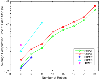
The principle behind is more worthy of discussion. Since there has been no explicit conclusion on complexity of Mixed Integer Programming so far, we conduct the complexity analysis based on the number of variables and constraints used by CMPC and HMPC. By replacing the state equations and input constraints, input variables and intermediate state variables treated by a central controller in CMPC with the reachable set, the problem computer by the centralized controller of HMPC is much simpler. Furthermore, the optimization problem in each robot restricts to local state equations and input constraints in HMPC, whose scale is small. And all the problems are solved concurrently. So it is not surprised that HMPC requires much less time than CMPC.

When applied to real world problems, if the time given to the controller synthesis is too short, similar to existing heuristic-search methods, HMPC will let robots stop and wait at each collaboration instant, until the controller is derived. Also, the computation time can be further reduced by removing certain constraints in the central optimization problem. For example, collision avoidance constraints between robots that are not close to each other may be safely removed.

6 Conclusion

We propose a hierarchical Model Predictive Control (HMPC) for the navigation problem of linear dynamical multi-robot systems with no reference trajectory. Using reachable set function computed off-line, our proposed HMPC scheme can successfully decouple constraints in objective functions and constraints, thus allowing computation to be distributed to the local controller of each robot and to run in parallel. Therefore, HMPC is computationally more efficient than CMPC as evidenced by our simulation. On the other hand, while the DMPC schemes cannot always ensure feasibility and stability, HMPC can guarantee its feasibility and stability in the same way as CMPC, therefore can be more viable, which is also evidenced by our simulation. In essence, the proposed HMPC combines the merits from both CMPC and DMPC schemes. An immediate future work is to expand HMPC for multi-robot systems with non-linear dyamics.

Acknowledgement

This research is supported by National Key Basic Research Program of China (2014CB340703), National Natural Science Foundation of China (No.61561146394, No.61321491, No.61373033), Specialized Research Fund for the Doctoral Program of Higher Education (20110091120058), Project on the Integration of Industry, Education and Research of Jiangsu Province (BY2014126-03), SZSTI Project JCYJ201418193546117 and also by Collaborative Innovation Center of Novel Software Technology and Industrialization.