
State-Dependent Cost Partitionings for Cartesian Abstractions in Classical Planning
Proceedings of the Twenty-Fifth International Joint Conference on Artificial Intelligence. Pages 3161-3168.
Abstract
Abstraction heuristics are a popular method to guide optimal search algorithms in classical planning. Cost partitionings allow to sum heuristic estimates admissibly by distributing action costs among the heuristics. We introduce state-dependent cost partitionings which take context information of actions into account, and show that an optimal state-dependent cost partitioning dominates its state-independent counterpart. We demonstrate the potential of our idea with a state-dependent variant of the recently proposed saturated cost partitioning, and show that it has the potential to improve not only over its state-independent counterpart, but even over the optimal state-independent cost partitioning. Our empirical results give evidence that ignoring the context of actions in the computation of a cost partitioning leads to a significant loss of information.
- [Bäckström and Nebel, 1995] Christer Bäckström and Bern- hard Nebel. Complexity results for SAS + planning. Com- putational Intelligence, 11(4):625-655, 1995.
- [Bonet and van den Briel, 2014] Blai Bonet and Menkes van den Briel. Flow-based heuristics for optimal planning: Landmarks and merges. In Proc. ICAPS 2014, pages 47- 55, 2014.
- [Bryant, 1986] Randal E. Bryant. Graph-based algorithms for boolean function manipulation. IEEE Transactions on Computers, 35(8):677-691, 1986.
- [Ciardo and Siminiceanu, 2002] Gianfranco Ciardo and Radu Siminiceanu. Using edge-valued decision diagrams for symbolic generation of shortest paths. In Proceedings of the Fourth International Conference on Formal Meth- ods in Computer-Aided Design (FMCAD 2002), pages 256-273. Springer Berlin Heidelberg, 2002.
- [Culberson and Schaeffer, 1998] Joseph C. Culberson and Jonathan Schaeffer. Pattern databases. Computational In- telligence, 14(3):318-334, 1998.
- [Edelkamp, 2001] Stefan Edelkamp. Planning with pattern databases. In Proc. ECP 2001, pages 84-90, 2001.
- [Felner et al., 2004] Ariel Felner, Richard Korf, and Sarit Hanan. Additive pattern database heuristics. JAIR, 22:279-318, 2004.
- [Geißer et al., 2015] Florian Geißer, Thomas Keller, and Robert Mattmüller. Delete relaxations for planning with state-dependent action costs. In Proc. IJCAI 2015, pages 1573-1579, 2015. IJCAI
- [Geißer et al., 2016] Florian Geißer, Thomas Keller, and Robert Mattmüller. Abstractions for planning with state- dependent action costs. In Proc. ICAPS 2016, 2016. To appear. Haslum et al., 2007] Patrik Haslum, Adi Botea, Malte Helmert, Blai Bonet, and Sven Koenig. Domain- independent construction of pattern database heuristics for cost-optimal planning. In Proc. AAAI 2007, pages 1007- 1012, 2007.
- [Helmert and Mattmüller, 2008] Malte Helmert and Robert Mattmüller. Accuracy of admissible heuristic functions in selected planning domains. In Proc. AAAI 2008, pages 938-943, 2008.
- [Helmert, 2006] Malte Helmert. The Fast Downward plan- ning system. JAIR, 26:191-246, 2006.
- [Karpas and Domshlak, 2009] Erez Karpas and Carmel Domshlak. Cost-optimal planning with landmarks. In Proc. IJCAI 2009, pages 1728-1733, 2009. IJCAI
- [Katz and Domshlak, 2007] Michael Katz and Carmel Domshlak. Structural patterns of tractable sequentially- optimal planning. In Proc. ICAPS 2007, pages 200-207, 2007.
- [Katz and Domshlak, 2010] Michael Katz and Carmel Domshlak. Optimal admissible composition of abstrac- tion heuristics. AIJ, 174(12-13):767-798, 2010.
- [Keller et al., 2016] Thomas Keller, Florian Pommerening, Jendrik Seipp, Florian Geißer, and Robert Mattmüller. State-dependent cost partitionings for cartesian abstrac- tions in classical planning: Full proofs. Technical Report CS-2016-002, University of Basel, Department of Mathe- matics and Computer Science, 2016.
- [Korf and Felner, 2002] Richard E. Korf and Ariel Felner. Disjoint pattern database heuristics. AIJ, 134(1-2):9-22, 2002.
- [Lai et al., 1996] Yung-Te Lai, Massoud Pedram, and Sarma B. K. Vrudhula. Formal verification using edge-valued bi- nary decision diagrams. IEEE Transactions on Computers, 45(2):247-255, 1996.
- [Pommerening et al., 2015] Florian Pommerening, Malte Helmert, Gabriele Röger, and Jendrik Seipp. From non- negative to general operator cost partitioning. In Proc. AAAI 2015, pages 3335-3341, 2015.
- [Röger et al., 2014] Gabriele Röger, Florian Pommerening, and Malte Helmert. Optimal planning in the presence of conditional effects: Extending LM-Cut with context split- ting. In Proc. ECAI 2014, pages 80-87, 2014.
- [Rudell, 1993] Richard Rudell. Dynamic variable ordering for ordered binary decision diagrams. In Proc. ICCAD 1993, pages 42-47, 1993.
- [Seipp and Helmert, 2013] Jendrik Seipp and Malte Helmert. Counterexample-guided Cartesian abstrac- tion refinement. In Proc. ICAPS 2013, pages 347-351, 2013.
- [Seipp and Helmert, 2014] Jendrik Seipp and Malte Helmert. Diverse and additive Cartesian abstraction heuristics. In Proc. ICAPS 2014, pages 289-297, 2014.
References were extracted automatically from the PDF and may contain errors.
Full text extracted automatically from the PDF; figures, tables and equations may differ. The PDF is the version of record.
1 Introduction
Abstraction heuristics based on pattern databases [Culberson and Schaeffer, 1998; Edelkamp, 2001] or the more general Cartesian abstractions [Seipp and Helmert, 2013] are popular methods to guide optimal heuristic search algorithms in classical planning. Since a single abstraction often provides poor guidance in challenging problems [Helmert and Mattm¨uller, 2008], we would like to combine the information from several abstractions admissibly. The simplest approach maximizes over a set of admissible heuristics. However, even though this often improves over the heuristic of a single abstraction, it does not really combine information of different sources but rather just selects the most accurate one.
Additive pattern databases [Korf and Felner, 2002; Felner et al., 2004] are one technique for combining information from a set of abstractions. They are based on the idea that heuristic estimates can be added up and still form an admissible heuristic as long as the used abstractions are pairwise independent. The related canonical heuristic [Haslum et al., 2007] combines both ideas: for a given set of abstractions, it computes all maximal subsets of pairwise independent abstractions and the sum of their heuristic values, and uses the maximum of these values to estimate the goal distance from a given state.
Cost partitioning [Katz and Domshlak, 2007; 2010] generalizes additive heuristics by replacing the requirement that the cost of each action may only be considered in a single abstraction with the requirement that the accumulated cost of each action over all abstractions may not exceed the original cost. Karpas and Domshlak [2009], for instance, distribute action costs among sub-tasks derived from a set of landmarks. In the context of Cartesian abstractions, Seipp and Helmert [2014] introduced saturated cost partitioning, where a cost partitioning is computed iteratively by "consuming" the minimum costs in each abstraction such that the costs of all shortest paths are preserved. Finally, general cost partitioning [Pommerening et al., 2015] extends the formalism to allow negative costs, which leads to admissible estimates that can be higher than an optimal cost partitioning restricted to non-negative costs.
In this paper, we show that even more information can be extracted from an abstraction collection if context information is used. Accounting for complete context information corresponds to computing a cost partitioning over all transitions - or, equivalently, over all state-action pairs - rather than only over all actions. We define the concept of statedependent cost partitionings and show that an optimal one dominates the optimal state-independent cost partitioning.
As the saturated state-independent cost partitioning maximizes over all transitions incurred by the same action, it loses valuable information. We show that the saturated statedependent cost partitioning, where costs are consumed only in a given context, does not suffer from this loss of information. Our implementation follows the idea of Geißer et al. [2016] who use edge-valued multi-valued decision diagrams (EVMDDs) [Ciardo and Siminiceanu, 2002] to encode context information efficiently. Even though saturated state-dependent cost partitioning does not dominate optimal nor saturated state-independent cost partitioning, it has the potential to produce better heuristic estimates than both. A preliminary experimental evaluation shows that the concept is relevant in practice and able to improve heuristic estimates
2 Background
Planning Tasks. We consider SAS+ planning tasks [B¨ackstr¨om and Nebel, 1995] with state-independent action costs, where a planning task is given as a tuple ⇧ = (V↪ A↪ sI ↪ s?↪ c) that consists of the following components: V is a finite set of state variables v, each with an associated finite domain Dv. A fact is a pair (v↪ d), where v 2 V and d 2 Dv, and a partial variable assignment s over V is a set of facts that belong to different variables. If s assigns a value to each v 2 V, s is called a state. We use function notation s(v) = d and set notation (v↪ d) 2 s interchangeably and denote the set of states of ⇧ with S. Each action a = hpre↪ effi in the set of actions A is a pair of partial variable assignments, called precondition and effect. The state sI 2 S is called the initial state, and the partial variable assignment s? specifies the goal condition. A state s is a goal state if s? ✓ s. We denote the set of goal states by S?.
An action a is applicable in state s iff pre ✓ s. Applying a in s yields the state s0 with s0 (v) = eff(v) where eff(v) is defined and s0 (v) = s(v) otherwise. We write s[a] for s0 . The (non-negative) cost of applying a is given by the cost function c : A ! R+0 of ⇧ as c(a). However, at several places in this paper, we are interested in costs that are based on altered cost functions. An important aspect of this work are general and state-dependent cost functions c : A⇥ S ! R that determine transition costs c(a↪ s) that depend on the state s in addition to the action a that is applied. Since state-dependent cost functions are more general, we define the following concepts in terms of state-dependent instead of regular cost functions unless we want to emphasize that the cost function of the original task is used. The resulting framework is similar to the formalism introduced by Geißer et al. [2015] for SAS+planning tasks with state-dependent action costs.
Let ⇡ = ha1↪ ▷ ▷ ▷ ↪ ani be a sequence of actions from A. We call ⇡ applicable in s0 if there exist states s1↪ ▷ ▷ ▷ ↪ sn such that ai is applicable in si-1 and si = si-1[ai] for all i = 1↪ ▷ ▷ ▷ ↪ n and write s[⇡] for sn. We call ⇡ an s-plan for ⇧ if it is applicable in s and if sn 2 S?. The cost of an s0-plan ⇡ under cost function c is the sum of action costs along the induced state sequence, i.e., c(⇡) = Pni=1 c(ai↪ si-1). An optimal s-plan under c is an s-plan that minimizes c(⇡). Its cost is denoted by h? (s↪ c). If there is no s-plan then h? (s↪ c) = 1. A heuristic function h estimates the cost of an optimal s-plan under cost function c with values h(s↪ c) 2 R [ ¶-1↪1♦. Note that we allow negative heuristic values to support general cost partitioning [Pommerening et al., 2015]. A heuristic h is called admissible if it never overestimates the true cost, i.e., h(s↪ c) h? (s↪ c) for all states s 2 S.
A planning task ⇧ and a cost function c induce a transition system T = (S↪ L↪ T↪ sI↪ S?) with state space S, transition labels L, transition relation T, initial state sI and goal states S? as usual, except that besides source state s, target state t and transition label a, transitions in T also carry a weight w 2 R, which is determined by s and a as w = c(s↪ a). For transitions we also write s a↪w --! t. It follows that a plan for s is a path from s to some sn 2 S? and the plan is optimal if the sum of the weights along the path is minimal.
Cartesian Abstractions. The core idea of abstraction heuristics is to collapse several states into a single abstract state, which reduces the size of the transition system and allows the computation of goal distances that can be used as admissible heuristic estimates. Given a planning task ⇧ with induced transition system T = (S↪ L↪ T↪ sI↪ S?), let ↵ be an equivalence relation on S that describes equivalence classes of the form D1 ⇥ D2 ⇥ · · · ⇥ Dn, where Di ✓ Dvi for V = ¶v1↪ ▷ ▷ ▷ ↪ vn♦. The resulting abstract states are often called Cartesian abstract states, but since we only consider Cartesian abstractions, we call them abstract states in the following. T and ↵ induce an abstract transition system T ↵ = (S↵↪ L↪ T ↵↪ ↵(sI)↪ S↵ ? ) in the following way: each concrete state s is mapped to the abstract state ↵(s) 2 S↵; the initial state sI is mapped to the abstract initial state ↵(sI) and goal states are mapped to abstract goal states S↵ ? = ¶↵(s?) ♣ s? 2 S?♦; there is a labelled abstract transition between ↵(s) and ↵(s0 ) whenever there is a concrete transition with the same label between s and s0 .
As long as action costs are state-independent, the weight of an abstract transition is simply the cost of the concrete action that induces it. In the presence of state-dependent action costs (which are not present initially in our input tasks, but can be introduced by state-dependent cost partitionings), determining the weight of an abstract transition is not as straightforward. Geißer et al. [2016] define the weight of an abstract transition between abstract states t and u with transition label a to be the minimal weight of all concrete transitions labeled with action a that start in a state s with ↵(s) = t. Together with the fact that every plan in the concrete transition system is a plan in the abstract transition system, this definition ensures that the cost of each abstract plan may be used as an admissible heuristic estimate. For now, the definition of Geißer et al. is sufficient for our needs, but we present an enhanced method in Section 6 that estimates abstract transition weights more precisely, while still guaranteeing admissibility.
3 Running Example
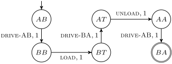
Throughout the paper, we use a simple logistics task as a running example, where a truck that starts in location A has to fetch a package from location B and bring it to A. The truck must return to B after the delivery. The corresponding transition system is given in Figure 1.
The task is described by two variables V = ¶T↪ P♦ that encode the position of the truck and the package, respectively.
The truck can be in each of the two locations (DT = ¶A↪ B♦) and the package can be in either location or in the truck (DP = ¶A↪ B↪ T♦). The truck can drive without load from A to B (DRIVE-AB) and with load from B to A (DRIVE-BA). There are actions to LOAD the package into the truck in B or UNLOAD it from the truck in A. All actions have unit cost.
Note that we explicitly exclude all other actions such as driving from B to A without the package or unloading the package at B. While this makes the task trivially solvable, the task is still sufficient to show some interesting properties.
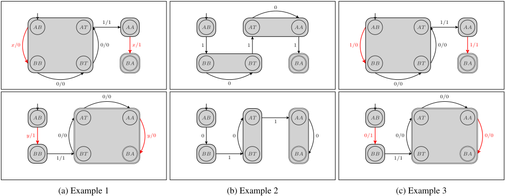
Figure 2 shows three pairs of abstractions for our example task which are used in the remainder of this paper. In all examples, we assume that the applied heuristic is the goal distance function in each abstraction, denoted h1 and h2, respectively. Additionally, since all concrete states have exactly one applicable action, we also refer to state-action pairs (a↪ s) as s!. Given cost function c, we write c(s!) for c(a↪ s).
4 State-dependent Cost Partitioning
Early work on additive admissible heuristics has mostly focused on techniques that allow to generate or identify heuristics that can be added up admissibly because each deals with a sub-problem of the planning task that can be regarded independently from the rest [Felner et al., 2004; Haslum et al., 2007]. An equivalent view on these techniques is to regard them as cost partitionings [Katz and Domshlak, 2007; 2010] that distribute action costs such that each operator is assigned its full cost in one heuristic and a cost of zero in all other. However, cost partitionings are more general as costs can be distributed arbitrarily between the heuristics as long as the sum over the individual costs does not exceed the original cost. Given such a cost partitioning, heuristic values are then computed on a copy of the planning task where actions cost only the fraction of the actual action cost that is assigned to the heuristic. Recently, Pommerening et al. [2015] showed that the framework can be extended from non-negative to general cost partitioning, which often allows to derive more accurate heuristic functions.
In this paper, we continue the process of developing more accurate cost partitioning techniques by presenting statedependent cost partitionings, a generalization where context information of applied actions is additionally taken into account.
Definition 1. Let ⇧ be a planning task. A (general) statedependent cost partitioning for ⇧ is a tuple P = hc1 ▷ ▷ ▷ ↪ cni, where ci : A⇥ S ! R for 1 i n and Pni=1 ci(a↪ s) c(a) for all s 2 S and a 2 A. If P is state-independent, i.e., such that ci(a↪ s) = ci(a↪ s0 ) for all s↪ s0 2 S, a 2 A and 1 i n, we call P a general state-independent cost partitioning for ⇧.
The introduction of state-dependent cost functions does not change the fact that admissible additive heuristic can be derived.
Theorem 1. Let h1↪ ▷ ▷ ▷ ↪ hn be admissible heuristics for a planning task ⇧ and P = hc1 ▷ ▷ ▷ ↪ cni be a state-dependent cost partitioning for ⇧. Then hP (s) = Pni=1 hi(s↪ ci) is an admissible heuristic. If any term in the sum is 1, the sum is defined as 1, even if another term is -1.
Proof sketch: The proof is a straightforward extension of the corresponding proof for state-independent cost partitionings (Theorem 1 in the work of Pommerening et al., 2015). It can be found in the technical report [Keller et al., 2016].
State-dependent cost partitionings differ from their stateindependent counterpart in the fact that each state-action pair can have its own cost instead of a cost that is shared among all possible applications of an action. If abstraction heuristics are considered, this corresponds to transition systems where all transitions can have arbitrary weights on the one hand and transition systems where all transitions with the same label share the same weight on the other.
Definition 2. Let h1↪ ▷ ▷ ▷ ↪ hn be admissible heuristics for a planning task ⇧, PD the space of possible state-dependent cost partitionings and PI ✓ PD the space of possible stateindependent cost partitionings for ⇧. The optimal statedependent cost partitioning (OCPD) heuristic estimate for h1↪ ▷ ▷ ▷ ↪ hn in state s is hocp D(s) = maxP2PD hP (s), and the optimal state-independent cost partitioning (OCPI) heuristic estimate for h1↪ ▷ ▷ ▷ ↪ hn is hocp I (s) = maxP2PI hP (s).
State-dependent cost partitionings allow the computation of more accurate heuristics estimates, which is the most important theoretical contribution of this paper.
Theorem 2. Let h1↪ ▷ ▷ ▷ ↪ hn be admissible heuristics for a planning task ⇧. For all s 2 S it holds that hocp D(s) ≥ hocp I (s). Moreover, there are planning tasks where the inequality is strict for at least one state.
Proof: The statement that hocp D(s) ≥ hocp I (s) for all s 2 S holds as every state-independent cost partitioning is also a state-dependent cost partitioning. The second statement follows from the following example.
Example 1. Consider the two abstract transition systems T1 and T2 in Figure 2a. The first edge label denotes the cost assigned by OCPI, and the second the cost assigned by OCPD. If an action induces only self-loops (depicted by dotted arcs) in one abstraction and must be part of a shortest path (depicted by solid arcs) in the other such as AT ! and BB!, all optimal cost partitionings use their full cost in the abstraction where the transition is part of the path. The difference between OCPI and OCPD is the distribution of the cost of action DRIVE-AB, which induces the two transitions AB! and AA! in our example task.
State-independent cost partitionings must assign the same value to both transitions within each abstraction. Let this value be x for the first and y for the second abstraction in our example. The heuristic value of the initial state under an optimal state-independent cost partitioning is then the maximum of (1 + x) + (y + 1) subject to x + y 1, so hocp I (AB) = 3.
State-dependent cost partitionings, on the other hand, allow that two transitions that are induced by the same action are assigned different costs within the same abstraction - as long as the sum of assigned costs for each transition does not exceed that transitions original cost. In our example, a possible optimal state-dependent cost partitioning is to assign the full cost to AA! in the first and to AB! in the second abstraction, which combines to a heuristic value of hocp D (AB) = 2 + 2 = 4
Even though Theorem 2 provides an encouraging result, its practical impact is limited without further work. This is mostly because the computation of an optimal statedependent cost partitioning with a method that is used to compute a state-independent cost partitioning [Katz and Domshlak, 2010; Bonet and van den Briel, 2014; Pommerening et al., 2015] would require a compilation with one action for each state-action pair, a number that is linear in the number of states and hence exponential in the number of variables. Even though there are techniques like context splitting [R¨oger et al., 2014] that allow to compute a more compact compilation, the worst-case exponential blowup cannot be avoided in general. We therefore turn our attention to saturated cost partitioning [Seipp and Helmert, 2014], a cost partitioning that is tractable in practice.
5 Saturated Cost Partitioning
Seipp and Helmert [2014] introduced the concept of cost saturation. Iteratively, they compute an abstraction, reduce the action costs such that all goal distances are preserved, and use the remaining costs for subsequent abstractions. The result is known as a saturated cost partitioning. Due to the greedy nature of the procedure, the resulting cost partition usually provides worse estimates than the optimal cost partition. However, we can compute the saturated cost partitioning much faster and do not need to hold all abstractions in memory simultaneously.
Saturated State-independent Cost Partitioning. In order to show that saturated cost partitioning yields an admissible heuristic even in the presence of general costs, we extend the underlying lemma from the original paper to general costs.
Lemma 1 (Lemma 5 of Seipp and Helmert [2014] extended to general costs). Let h and h0 denote the goal distance functions in two transition systems T and T 0 that differ only in the weight of a single transition s ! s0 , which is w 2 R in T and w0 2 R in T 0 . If h(s) - h(s0 ) w0 w↪ then h = h0 .
Proof sketch: We only sketch this proof here and refer to the technical report [Keller et al., 2016] for a full proof.
The only difference to Lemma 5 of Seipp and Helmert [2014] is that we allow general costs and hence negative weights in transition systems. With their proof, it is easy to see that negative weights are unproblematic unless there is a negative-cost cycle including the transition s ! s0 in T 0 but not in T (because then h(s0 ) 6= h0 (s0 )). Assume there is a cyclic path s w -! s0 d-!⇤ s, that is only negative in T 0 , i.e. w + d > 0 and w0 + d < 0. Since h estimates goal distances, we get h(s0 ) h(s) + d and hence 0 h(s) - h(s0 ) + d. However, from h(s) - h(s0 ) w0 and w0 + d < 0, we get h(s) - h(s0 ) + d < 0, which is a contradiction.
With the preceding lemma we can define saturated stateindependent cost partitioning for general costs while preserving admissibility.
Definition 3. Let ⇧ be a planning task with cost function c and ↵1↪ ▷ ▷ ▷ ↪ ↵n abstractions. Let hc1↪ ▷ ▷ ▷ ↪ cni and P = hˆ c1↪ ▷ ▷ ▷ ↪ ˆ cni be tuples of cost functions with the following properties: c1 = c; ˆ ci(a) = maxs2S hi(↵i(s)) - hi(↵i(s[a])), where hi is the goal distance function of T ↵i with cost function ci; and ci+1 = ci - ˆ ci. We call ci the remaining cost for T ↵i , ˆ ci the saturated cost of T ↵i and P the saturated state-independent cost partitioning for ↵1↪ ▷ ▷ ▷ ↪ ↵n.
We denote the associated heuristic by hscp I . Seipp and Helmert [2014] show that the saturated cost function preserves the goal distances of all abstract states in all abstractions, and is minimal among all distance-preserving cost functions. Next, we illustrate the computation of SCPI in our example domain.
Example 2. Consider the two abstract transition systems of our running example that are shown in Figure 2b. The goal distances of T1 are h1(¶AB♦) = 3, h1(¶BB↪BT♦) = 2, h1(¶AT↪AA♦) = 1, and h1(¶BA♦) = 0. The saturated cost ˆ c1 of T1, which annotates the edge labels, assigns the full cost of 1 to both DRIVE-AB (which induces both AB! and AA!) and DRIVE-BA (i.e., BT !), and 0 to all other actions. The remaining costs c2, which are used to compute the goal distances in T2, are hence 0 for all actions except c2(BB!) = c2(AT !) = 1. With this, the saturated stateindependent cost partitioning for the initial state of our example is hscp I (AB) = 3 + 2 = 5.
Saturated State-dependent Cost Partitioning. As stateindependent cost functions do not allow that costs are assigned to actions in the context of the current state, saturated cost functions are computed by maximizing over all weights of transitions that are labeled with the same action. Statedependent cost partitioning offers an opportunity to overcome this weakness by allowing to reduce the costs of state-action pairs rather than actions.
Definition 4. Let ⇧ be a planning task with cost function c and ↵1↪ ▷ ▷ ▷ ↪ ↵n abstractions. Let hc1↪ ▷ ▷ ▷ ↪ cni and P = hˆ c1↪ ▷ ▷ ▷ ↪ ˆ cni be tuples of cost functions with the following properties: c1(a↪ s) = c(a) for all a 2 A and s 2 S; ˆ ci(a↪ s) = hi(↵(s)) - hi(↵(s[a])), where hi is the goal distance function of T ↵i with cost function ci; and ci+1 = ci - ˆ ci. We call ci the remaining cost for T ↵i , ˆ ci the saturated cost of T ↵i and P the saturated state-dependent cost partitioning for ↵1↪ ▷ ▷ ▷ ↪ ↵n.
We denote the associated heuristic by hscp D . Let us investigate the differences between both versions of cost saturation.
Example 3. Consider the two abstract transition systems in Figure 2c, where the first transition label denotes the goal distances of SCPI and the second the goal distances of SCPD. Due to the state-independence of SCPI, a cost of 1 is assigned to both occurrences of DRIVE-AB in the first abstraction, such that no cost is left in the second one and hscp I (AB) = 2 + 1 = 3. Because SCPD is state-dependent, the cost of AB! can be used in the second abstraction and the heuristic estimate is hscp D (AB) = 2 + 2 = 4.
In analogy to Theorem 2, Example 3 hints at a theoretical dominance of SCPD over SCPI. However, it turns out that this is not the case due to the inaccuracy caused by the greedy nature of saturated cost partitionings.
Theorem 3. There are planning tasks ⇧ and ⇧0 with states s 2 S and s0 2 S0 such that hscp D(s) > hscp I (s) and hscp I (s0 ) > hscp D (s0 ).
Proof sketch: Example 3 shows that there are instances where hscp D(s) > hscp I (s). For hscp I (s) > hscp D(s), consider the following example.
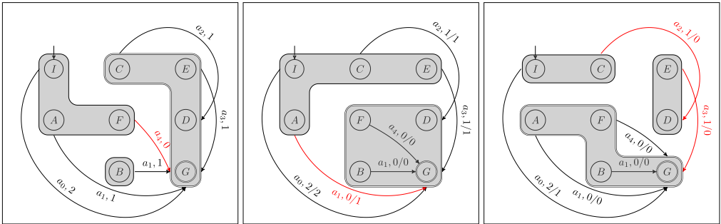
Example 4. Consider the planning task and the three abstract transition systems that are shown in Figure 3. The abstractions in the example are not Cartesian, which is necessary to keep it small. An example that follows the same idea but uses Cartesian abstractions is contained in the technical report [Keller et al., 2016].
First, consider the state-independent case (first label in the figure): in T1, only the cost of a1 is required to maintain the heuristic values, i.e., the saturated cost of T1 is ˆ c1(a1) = 1 and 0 for all other actions. The remaining cost of a1 for T2 thus is 0, so the abstract initial state has a heuristic value of 0 in T2 and the saturated cost of T2 is 0 for all actions. Since a0, a2, and a3 all still have their original cost in T3, the abstract initial state of T3 has a heuristic value of 2. Therefore, the overall heuristic value is hscp I (I) = 0 + 0 + 2 = 2.
Now consider the state-dependent case (second label in the figure): here, the saturated cost of T1 is ˆ c1(a1↪B) = 1 but ˆ c1(a1↪A) = 0, so the remaining cost for T2 is c2(a1↪A) = 1 and the heuristic value for the abstract initial state of T2 is 1 instead of 0. This means that the saturated cost of T2 is ˆ c2(a0↪ I) = ˆ c2(a1↪A) = ˆ c2(a2↪C) = ˆ c2(a3↪E) = 1 and 0 for all other actions, and that no cost remains for a2 and a3 in T3. Therefore, the overall heuristic value is hscp D(I) = 0 + 1 + 0 = 1 < 2 = hscp I (I).
In Theorems 2 and 3 we have investigated the relationship between OCPD and OCPI on the one hand and SCPD and SCPI on the other. What is left is the relationship between SCPD and OCPI.
Corollary 1. There are a planning tasks ⇧ and ⇧0 with states s 2 S and s0 2 S0 such that hscp D(s) > hocp I (s) and hocp I (s0 ) > hscp D (s0 ).
Proof: For the first part, consider Examples 1 and 3 where hscp D(AB) = 4 and hocp I (AB) = 3. The second part follows from Definition 2 and Theorem 3.
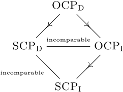
Figure 4 shows a summary of our theoretical results (where A ≻ B means A dominates B). While optimal statedependent cost partitioning clearly combines the best of both worlds, we leave it for future work, since computing it is exponential. On the other hand, saturated state-dependent cost partitioning may not always result in better heuristic estimates, but it has the potential to surpass optimal stateindependent cost partitioning, which warrants further investigation. We therefore discuss practical considerations for the computation of saturated state-dependent cost partitioning in the following section.
6 Implementation Details of hscp D
Given a set of abstractions, Section 5 reveals a general workflow to compute saturated state-dependent cost partitionings. For each abstraction we have to apply the following four steps: (1) determine the abstract transition weights (with the current remaining cost function), (2) compute the abstract goal distances, (3) compute the saturated state-dependent cost function, and (4) determine the remaining cost function. Note that the cost function for the first abstraction is the (stateindependent) original cost function, while subsequent abstractions use the remaining costs, computed in the previous iteration. In general, it is not important howwe obtain the abstractions, although some abstractions or abstraction orders may result in better heuristics than others. We will briefly discuss this in Section 7. In fact, we do not even require Cartesian abstractions. When we describe the implementation of the four steps above in the remainder of this section, we will, however, see that Cartesian abstractions are necessary to guarantee some important properties.
Edge-valued Decision Diagrams. To encode statedependent cost functions, we need a suitable representation. We chose edge-valued multi-valued decision diagrams, because they are (i) often compact, albeit worst-case exponential, they (ii) allow efficient computation of abstract cost values as long as the abstract states are Cartesian [Geißer et al., 2016], and they (iii) admit reasonably efficient arithmetic operations, in particular subtraction of the current saturated costs from the current remaining costs that is needed to determine the remaining costs for the next iteration. Taking binary sums and differences is linear in the product of the sizes of the input EVMDDs, a result that can be easily generalized from a result by Lai et al. [1996] on EVBDDs. EVMDDs work as follows: like BDDs [Bryant, 1986], EVMDDs contain decision nodes. At each decision node, the diagram branches over the value of the associated decision variable. There are three differences from BDDs: first, branchings can be n-ary instead of only binary, second, the values returned by evaluating an EVMDD can come from a finite range of values instead of just being true or false, and third, the return values are associated with the edges of the diagram instead of the leaves. When traversing an EVMDD for a single valuation s, the resulting value is the sum of edge weights along the unique path corresponding to s.
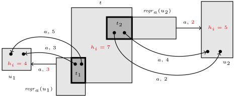
Determining Abstract Transition Weights. Assume that we have an EVMDD representing the remaining cost function for the current abstraction of some action a, and that we want to use this EVMDD to determine abstract transition weights for the next abstraction we build. The main challenge is this: with the EVMDD, we can easily determine what a costs in any concrete state. Geißer et al. [2016] show that we can use the same EVMDD to efficiently determine what a costs in any abstract state as well, as long as the abstract state is Cartesian. Here, we extend their technique in order to obtain more accurate transition weights depending not only on the source state of the transition, but also on its target state. Note that for deterministic transition systems, this does not make a difference, but for non-deterministic transition systems it does, and that the abstractions we consider here may indeed introduce non-determinism. More specifically, we want to be able to assign two different weights to two different abstract transitions t a-! u1 and t a-! u2 with the same abstract source state t and the same action label a depending on whether it leads to u1 or u2. This gives us more accurate abstract goal distances. In order to accomplish this, we (i) identify via regression the subset t1 of t where a is applicable and leads to u1, and (ii) restrict t to that subset; and similarly for u2. Both regression and intersection of Cartesian sets preserve Cartesianness [Seipp and Helmert, 2013], so we can still safely assume that t1 and t2 are Cartesian sets and hence admit efficient EVMDD operations. Note that any two such t1↪ t2 that are computed by regression are indeed disjoint, even if they originate from the same abstract state t via regression through the same action a from two different states u1 and u2. Figure 5 illustrates the idea of improving the abstraction via regression. The abstract state t contains four concrete states where a is applicable, at costs 2, 3, 4, and 5, respectively. Simply minimizing the cost of a over all four states would require us to assign cost 2 to a in the entire set t. However, by partitioning the four concrete states into the two states leading to successors in u1 at cost 3 and 5 (represented by the Cartesian set t1), and into those two states leading to successors in u2 at cost 2 and 4 (represented by the Cartesian set t2), we can now assign cost 2 to a in t2, and the higher cost of 3 to a in t1.
Computing Saturated State-dependent Cost Functions.
Computing abstract goal distances is straightforward, e. g., using Dijkstra's algorithm in a backward manner. We skip discussing that and move on to computing saturated statedependent cost functions. We already know how to compute them from the theoretical part of this paper. Here, we discuss how to efficiently represent them using EVMDDs. Assume that after regression and saturation, action a costs δk in Cartesian set tk, k = 1↪ ▷ ▷ ▷ ↪m. Then we can obtain an EVMDD that encodes the saturated cost function of a as follows: for each set tk, we can efficiently compute an EVMDD that encodes the characteristic function of tk weighted with its cost δk. This EVMDD branches on all relevant variables in sequence, routing branches inconsistent with tk immediately to the sink and branches consistent with it to the next decision node/variable. All edge weights are zero except for those leading from the last decision variable to the sink that are consistent with tk. Those carry weight δk. Moreover, we can compute an EVMDD representing the sum of those characteristic-function EVMDDs for k = 1↪ ▷ ▷ ▷ ↪m, which is exactly the saturated cost function we are after. Taking this sum is exponential only in the number of Cartesian sets m and nothing else. In general, this cannot be avoided, not even in the Cartesian setting. Note that for abstract sets which do not lead to the goal we can assign sufficiently small saturated cost values to concrete states mapped to them. This results in arbitrarily large remaining costs, which mirrors the observation that applying the action in such a state makes the task unsolvable. Finally, representing the new remaining cost function of a as an EVMDD is trivial. We have EVMDDs for the previous remaining cost function and for the current saturated cost function of a. Taking the difference of two functions is a simple EVMDD operation and returns the desired EVMDD.
7 Empirical Evaluation
Even though the focus of this paper is on theoretical aspects of state-dependent cost partitionings, we have performed a brief empirical evaluation as well. Its aim is to investigate whether the potentially exponential blowup of the EVMDD size is critical in practice and how relevant state-dependent cost partitionings are in practice. It is important to note that we are not evaluating an elaborate algorithm that is optimized for the computation of accurate heuristic values with statedependent cost partitionings. The creation of abstractions that are well suited to be used in combination with statedependent cost partitionings is in particular not the focus of this paper, but plays an important role when accurate heuristic estimates are desired. Moreover, we did not implement any form of variable ordering in the decision diagrams [Rudell, 1993], which would further reduce their exponential blowup.
We have implemented the saturated state-dependent cost partitioning algorithm that is sketched in the previous section on top of the CEGAR implementation of Seipp and Helmert [2013] in the Fast Downward planning system [Helmert, 2006]. Our algorithms use the same parameter settings as the configuration that performed best for saturated stateindependent cost partitionings in the original work on the topic [Seipp and Helmert, 2014] with two exceptions: first, we used a maximal number of states (10000) instead of a timeout to decide when the heuristic computation terminates in order to make the abstraction generation process deterministic. And second, we do not interleave the generation of an abstraction based on the latest remaining cost function with the computation of its saturated cost function but compute all abstractions with the original cost function instead. Combined, both changes make sure that all algorithms compute their respective cost partitionings on identical abstract transition systems.
We have performed experiments on all supported IPC 1998-2014 benchmarks on Intel Xeon E5-2660 CPUs running at 2.2 GHz with a time limit of 30 minutes and a memory limit of 2 GB. The exponential blowup of the EVMDD size is critical in only six out of 57 domains, namely FREECELL, MPRIME, MYSTERY, PIPESWORLD-NOTANKAGE, PIPESWORLD-TANKAGE, and TIDYBOT 2011. However, a simple procedure that uses saturated state-independent costs for all abstractions where the number of transitions with nonzero cost is too large leads to an algorithm that preserves the advantages of state-dependent cost partitionings in most domains and mitigates the risk of unmanageable EVMDDs successfully.
Table 1 gives the number of instances per domain where the heuristic value of the initial state with hscp D is larger, smaller and derived from a different sum of heuristic values in comparison to hscp I . The state-dependent version improves over the state-independent one in 228 out of 1667 instances, it performs worse in 76, and there are another 25 instances where both compute the same heuristic estimate for the initial state but based on different sums. It is a promising result that hscp D is already better in approximately 17 of the instances even when the considered abstractions are not tailored to exploit context information. We believe that the fact that hscp I performs better on an instance is a sign that state-dependent costs are relevant in that instance, and it may very well only be the greediness of saturated cost partitionings, the poor abstraction generation or even just the abstraction order that prevent a result where hscp D is better than hscp I instead of worse.
Even when the estimates do not differ, we assume that it is often only the choice of abstractions that prevents an improved heuristic estimate with state-dependent cost partitionings. A look at the domains where the heuristic estimates differ in at least one instance reveals that similarly structured problems (like, for instance, route or transportation problems) are either present with a large number of representatives or not at all. This hints at the fact that the relevance of context information is domain- and not instance-dependent (i.e., relevant in all instances that are part of a domain with at least one instance were the heuristic estimates differ). Under the assumption that this is the case, there are 944 instances among the 1667 and hence more than half of them where state-dependent cost partitionings have the potential to improve over state-independent ones. We believe that this is a promising result that encourages future work on the topic, e.g., on well-suited abstraction generation methods or other state-dependent cost partitionings.
| Domain | hscpD > hscpI | hscpD < hscpI | different sum |
|---|---|---|---|
| AIRPORT (50) | 1 | 1 | 2 |
| BARMAN 2011 (20) | 16 | 0 | 16 |
| BARMAN 2014 (14) | 8 | 1 | 9 |
| BLOCKS (35) | 21 | 4 | 26 |
| DEPOT (22) | 4 | 3 | 7 |
| DRIVERLOG (20) | 1 | 5 | 7 |
| ELEVATORS 2008 (30) | 19 | 1 | 22 |
| ELEVATORS 2011 (20) | 12 | 1 | 15 |
| FLOORTILE 2011 (20) | 7 | 4 | 13 |
| FLOORTILE 2014 (20) | 7 | 5 | 14 |
| GRID (5) | 4 | 0 | 4 |
| HIKING 2014 (20) | 12 | 2 | 15 |
| MPRIME (35) | 1 | 0 | 2 |
| MYSTERY (30) | 0 | 0 | 1 |
| NOMYSTERY 2011 (20) | 4 | 1 | 5 |
| OPENSTACKS (30) | 2 | 0 | 2 |
| OPENSTACKS 2008 (30) | 10 | 0 | 10 |
| OPENSTACKS 2011 (20) | 6 | 0 | 6 |
| OPENSTACKS 2014 (20) | 3 | 0 | 3 |
| PARCPRINTER 2008 (20) | 7 | 1 | 8 |
| PARCPRINTER 2011 (20) | 5 | 1 | 6 |
| PARKING 2011 (20) | 0 | 1 | 1 |
| PATHWAYS-NONEG (30) | 3 | 16 | 22 |
| PSR-SMALL (50) | 11 | 0 | 11 |
| ROVERS (40) | 3 | 4 | 8 |
| SATELLITE (36) | 7 | 3 | 11 |
| SCANALYZER 2008 (30) | 1 | 0 | 1 |
| SCANALYZER 2011 (20) | 1 | 0 | 1 |
| SOKOBAN 2008 (30) | 6 | 0 | 6 |
| SOKOBAN 2011 (20) | 3 | 0 | 3 |
| TETRIS 2014 (17) | 1 | 1 | 2 |
| TPP (30) | 8 | 2 | 11 |
| TRANSPORT 2008 (30) | 14 | 4 | 20 |
| TRANSPORT 2011 (20) | 11 | 6 | 18 |
| TRANSPORT 2014 (20) | 9 | 9 | 18 |
| TRUCKS (30) | 0 | 0 | 1 |
| WOODWORKING 2008 (30) | 0 | 0 | 1 |
| WOODWORKING 2011 (20) | 0 | 0 | 1 |
| Remaining domains (723) | 0 | 0 | 0 |
| Total (1667) | 228 | 76 | 329 |
8 Conclusion
We generalized the concept of cost partitionings even further and showed that additional information can be extracted from a set of abstractions if context information of applied actions is taken into account. We showed that an optimal state-dependent cost partitioning dominates all stateindependent cost partitionings and that there are planning tasks where the dominance is strict. As it is unclear how an optimal state-dependent cost partitioning can be computed efficiently in practice, we applied the idea to the efficiently computable saturated cost partitioning. We showed that saturated state-dependent cost partitioning does not dominate its state-independent sibling, but may still surpass optimal stateindependent cost partitioning. We discussed practical considerations regarding saturated state-dependent cost partitioning and reasoned that EVMDDs are a suitable representation for the resulting cost functions as long as the abstractions are Cartesian. A baseline implementation of our approach revealed that there are indeed many instances among the IPC benchmarks where the heuristic estimates improve under a state-dependent cost partitioning. It furthermore allows to conjecture that taking context information into account can pay off in the majority of IPC benchmark tasks.
This work also opens up several possible directions for future work. Saturated state-dependent cost partitionings can be improved by reasoning about the order of the considered abstract transitions systems or with methods that generate Cartesian abstractions that are tailored to exploit context information. Dynamic variable orderings for decision diagrams are an enhancement that has the potential to further minimize the risk that an EVMDD's size gets out of hand. And finally, it should be possible to narrow the gap between the (errorprone) saturated state-dependent cost partitionings on the one hand and the optimal ones (which are intractable in practice) on the other. Context splitting, for instance, seems promising as it provides a tool that allows an iterative compilation of the input task, which might give rise to near-optimal statedependent cost partitionings in the future.
Acknowledgments
This work was supported by the European Research Council as part of the project "State Space Exploration: Principles, Algorithms and Applications" and by BMBF grant 02PJ2667 as part of the KARIS PRO project.
@inproceedings{ijcai2016p448,
  title     = {State-Dependent Cost Partitionings for Cartesian Abstractions in Classical Planning},
  author    = {Keller, Thomas and Pommerening, Florian and Seipp, Jendrik and Geißer, Florian and Mattmüller, Robert},
  booktitle = {Proceedings of the Twenty-Fifth International Joint Conference on
               Artificial Intelligence, {IJCAI-16}},
  publisher = {AAAI Press / International Joint Conferences on Artificial Intelligence},
  editor    = {Subbarao Kambhampati},
  pages     = {3161--3168},
  year      = {2016},
  month     = {7},
  url       = {https://ijcai.org/proceedings/2016/448},
}
TY - CPAPER TI - State-Dependent Cost Partitionings for Cartesian Abstractions in Classical Planning AU - Keller, Thomas AU - Pommerening, Florian AU - Seipp, Jendrik AU - Geißer, Florian AU - Mattmüller, Robert T2 - Proceedings of the Twenty-Fifth International Joint Conference on Artificial Intelligence, IJCAI-16 PB - AAAI Press / International Joint Conferences on Artificial Intelligence PY - 2016 SP - 3161 EP - 3168 UR - https://ijcai.org/proceedings/2016/448 ER -Copied
Machine-readable versions of this paper, for tools and AI agents:





