PAC Greedy Maximization with Efficient Bounds on Information Gain for Sensor Selection

1 Introduction

Submodularity is a property of set functions that formalizes the notion of diminishing returns i.e., adding an element to a set increases the value of the set function by a smaller or equal amount than adding that same element to a subset. Many realworld problems involve maximizing submodular functions, e.g., summarizing text [Li et al., 2012; Lin and Bilmes, 2010], selecting subsets of training data for classification [Chen and Krause, 2013], or selecting sensors to minimize uncertainty about a hidden variable [Satsangi et al., 2015].

Formally, given a ground set X = ¶1↪ 2 ▷ ▷ ▷ n♦, a set function F : 2X ! R, is submodular if for every AM ✓ AN ✓ X and i 2 X ∩ AN ,∆F (i♣AM ) ≥ ∆F (i♣AN )↪ (1)

where ∆F (i♣A) = F (A [ i) - F (A) is the marginal gain of adding i to A. Typically, the aim is to find an A⇤ that maximizes F subject to certain constraints. Here, we consider a constraint on A⇤ 's size: A⇤ = argmaxA✓X:♣A♣k F(A).

Frans A. Oliehoek

University of Liverpool University of Amsterdam frans.oliehoek@liverpool.ac.uk

As n increases, the (nk) possibilities for A⇤ grow rapidly, rendering naive maximization intractable. Instead, greedy maximization finds an approximate solution AG faster by iteratively adding to a partial solution the element that maximizes the marginal gain. Nemhauser et al. (1978) showed that the value obtained by greedy maximization is close to that of full maximization, i.e., F(AG) ≥ (1-e-1 )F(A⇤ ), if F is submodular, non-negative and monotone.

Lazy greedy maximization [Minoux, 1978] accelerates greedy maximization by pruning elements whose marginal gain on the last iteration ensures that their marginal gain on the current iteration cannot be maximal. Lazier greedy maximization [Mirzasoleiman et al., 2015] provides further speedup by evaluating the marginal gain only of a randomly sampled subset of elements at each iteration. Other variations [Wei et al., 2014; Badanidiyuru and Vondr´ak, 2014] also minimize the number of marginal gain computations.

However, these methods assume it is computationally feasible to exactly compute F, and thus the marginal gain. In many settings, this is not the case. For example, consider a surveillance task [Satsangi et al., 2015] in which an agent aims to minimise uncertainty about a hidden state by selecting a subset of sensors that maximise information gain. Computing information gain is computationally expensive, especially when the hidden state can take many values, as it involves an expectation over the entropy of posterior beliefs about the hidden state. When surveilling large areas like shopping malls, exactly computing the entropy of a single posterior belief becomes infeasible, let alone an expectation over them.

In this paper, we present a new algorithm called probably approximately correct greedy maximization. Rather than assuming access to F itself, we assume access only to confidence bounds on F. In particular, we assume that these bounds are cheaper to compute than F and are anytime, i.e., we can tighten them by spending more computation time, e.g., by generating additional samples. Inspired by lazy greedy maximization, our method uses confidence bounds to prune elements, thereby avoiding the need to further tighten their bounds. Furthermore, we provide a PAC analysis that shows that, with high probability, our method returns an approximately optimal set.

Given an unbiased estimator of F , it is possible to use concentration inequalities like Hoeffding's inequality to obtain the confidence bounds needed by PAC greedy maximization.

Unfortunately, many applications, such as sensor placement and decision tree induction, require information-theoretic definitions of F such as information gain. These definitions depend on computing entropy over posterior beliefs, which are impossible to estimate in unbiased way [Paninski, 2003]. The absence of an unbiased estimator renders Hoeffding's inequality inapplicable and makes it hard to obtain computationally cheap confidence bounds on conditional entropy [Nowozin, 2012; Loh and Nowozin, 2013]. Therefore, in this paper, we propose novel, cheap confidence bounds on conditional entropy.

Finally, we apply PAC greedy maximization with these new confidence bounds to a real-life dataset collected by agents controlling a multi-camera tracking system employed in a shopping mall. Our empirical results demonstrate that our approach performs comparably to greedy and lazier greedy maximization, but at a fraction of the computational cost, leading to much better scalability.

2 Background

Given a set function F : 2X ! R, greedy maximization [Nemhauser et al., 1978] computes a subset AG ✓ X that approximates A⇤ = arg maxA2A+ F (A), where A+ = ¶A ✓ X : ♣A♣  k♦. As shown in Algorithm 1, it does so by repeatedly adding to AG the element i that maximizes the marginal gain ∆F (i♣AG). Because it is greedy, this method is much faster than naive maximization.

Algorithm 1 greedy-max(F↪ X ↪ k)

Nemhauser et al. (1978) showed that, under certain conditions, this method has bounded error.

Theorem 1. (Nemhauser et al., 1978) If F is non-negative, monotone and submodular, then F(AG) ≥ (1-e-1 )F(A⇤ ).

Lazy greedy maximization [Minoux, 1978] accelerates greedy maximization by pruning elements whose marginal gain cannot be maximal by maintaining a priority queue of all elements in which each element's priority is its marginal gain computed in the previous iteration. If in the current iteration, the marginal gain of the element with the highest priority is higher than the priority of the next element, then the current iteration is terminated since submodularity guarantees that the marginal gain of the remaining elements can only decrease. Lazy greedy maximization computes the same AG as greedy maximization and is much faster in practice.

3 Problem Setting

In this paper, we consider a variation on submodular function maximization in which evaluating F, and therefore the marginal gain, is prohibitively expensive, rendering greedy and lazy greedy maximization inapplicable. Instead, we assume access to computationally cheap confidence bounds on F. In particular, let U and L be set functions such that for each A 2 A+, with probability 1 - δu, U(A) ≥ F(A) and for each A 2 A+, with probability 1 - δl, F(A) ≥ L(A). Furthermore, we assume that U and L are anytime, i.e., we have a tighten procedure that improves these bounds in exchange for computation. Specifically, calling tighten(A) will in expectation reduce U(A) and increase L(A).

These assumptions are easily satisfied in many settings where F is too expensive to compute exactly. For example, if F(A) = E[X♣A] for some random variable X, then ˆ F(A) = 1N (PNi=1 xi), where the xi's are i.i.d. samples of X, is an unbiased estimator of ˆ F (A) for which U and L can easily be constructed using, e.g., Hoeffding's inequality (1963). Furthermore, tighten need only fold more samples into ˆ F . However, we specifically do not assume access to ˆ F or any other unbiased estimator of F . Instead, we seek an algorithm that performs submodular function maximization given only U, L, and tighten.

The absence of an unbiased estimator of F arises in many settings in which F is defined using information-theoretic metrics such as information gain or entropy. For example, consider the sensor selection problem [Williams et al., 2007; Spaan and Lima, 2009] in which an agent has a set of sensors X = ¶1↪ 2 ▷ ▷ ▷ n♦ giving information about a hidden state s. For each sensor i, zi denotes the observation the agent will receive if it selects that sensor, with zi = ; if not selected. z = hz1↪ z2 ▷ ▷ ▷ zni denotes the complete observation vector generated by all sensors.

Upon selecting sensors A and observing z, the agent can compute a posterior belief using Bayes rule:

where Pr(z♣b↪A) = Ps b(s)Pr(z♣s↪A) and b(s) is a prior belief. The agent aims to minimize its uncertainty about s, measured as the entropy of b(s): Hb(s) = - Ps b(s) log(b(s))▷ Given b and A, the conditional entropy is:

where ⌦ is the set of all possible values of z that can come from sensors present in the set A. The agent's goal is to find A⇤ that maximizes information gain:

Since the first term in (4) is independent of A, we equivalently define F(A) as:

Unfortunately, when there are many possible states and actions, computing HbAz (s) is not only intractable, but also difficult to efficiently estimate [Paninski, 2003; Nowozin, 2012; Sch¨urmann, 2004]. In fact, Paninski (2003) showed that no unbiased estimator for entropy exists.

Therefore, in the next section we propose a new fundamentally different method that requires only U, L, and tighten. To solve sensor selection in particular, we also need cheap anytime implementations of U and L for conditional entropy, which we propose in Section 6.

4 Method

In this section, we propose probably approximately correct greedy maximization, which enables an agent to perform submodular function maximization without ever computing F exactly. The main idea is to use U and L to prune elements that with high probability do not maximize marginal gain.

Our approach is inspired by lazy greedy maximization. To see how, it is helpful to view lazy greedy maximization as a pruning method: terminating an iteration before the priority queue is empty effectively prunes each element whose upper bound (given by its marginal gain on the previous iteration) is lower than the maximum lower bound (given by the best marginal gain found so far on the current iteration).

PAC greedy maximization generalizes this idea in two ways. First, it accepts arbitrary upper and lower bounds. This makes it possible to replace the bounds used by lazy greedy maximization, which rely on exact computation of marginal gain, with cheaper ones. Second, it uses confidence bounds instead of hard bounds. By tolerating a small probability of error, our approach can prune more aggressively, enabling large speedups while maintaining a PAC bound.

Algorithm 2 pac-greedy-max(U↪ L↪ X ↪ k↪ ✏1↪ t) AP ; for m = 1 to k do AP AP [ pac-max(U↪ L↪AP ↪ ✏1↪ t) end for return AP

Algorithm 2 shows the main loop, which simply adds at each iteration the element selected by the pac-max subroutine. Algorithm 3 shows this subroutine, which maintains a queue of unpruned elements prioritized by their upper bound. In each iteration of the outer while loop, pac-max examines each of these elements and prunes it if its upper bound is not at least ✏1 greater than the max lower bound found so far. In addition, the element with the max lower bound is never pruned. If an element is not pruned, then its bounds are tightened. Algorithm 3 terminates when only one element remains or when the improvement produced by tightening U and L falls below a threshold t.

Algorithm 3 is closely related to best arm identification algorithms [Audibert and Bubeck, 2010] for multi-armed bandits. The main difference is that it does not directly estimate F. Instead, it selects an element using only U and L. In cases where an unbiased sample-based estimator of F is available, pac-max can be replaced by an off-the-shelf best arm identification algorithm that uses, e.g., Hoeffding bounds instead of U and L. However, in this paper, we focus on the setting in which no such estimator is available and thus bandit-based algorithms cannot be directly applied.

Algorithm 3 pac-max(U↪ L↪ AP ↪ ✏1↪ t)

iP 0 % element with max lower bound for i 2 X ∩ AP do ⇢▷enqueue(i↪ U(AP [ i)) % initial priority iP argmaxj2¶i↪iP ♦ L(AP [ j)♦ end for while ⇢▷length() > 1 _ change in U & L is > t do ⇢0 empty queue while ≻⇢▷empty() do i ⇢▷dequeue() if i = iP _ U(AP [ i) ≥ L(AP [ iP ) + ✏1 then tighten(AP [ i) iP argmaxj2¶i↪iP ♦ L(AP [ j) ⇢0 ▷enqueue(i↪ U(AP [ i)) end if end while ⇢ ⇢0 end while return iP

5 PAC Bounds

In this section, we analyze PAC greedy maximization. With oracle access to F , greedy maximization is guaranteed to find AG such that F(AG) ≥ (1 - e-1 )F(A⇤ ), if F is monotone, non-negative and submodular [Nemhauser et al., 1978]. Since PAC greedy maximization does not assume oracle access to F and instead works with cheap anytime confidence bounds on F, we prove a PAC bound for PAC greedy maximization. In particular, we prove that under the same conditions, PAC greedy maximization finds a solution AP such that, with high probability, F(AP ) is close to F(A⇤ ).

Since greedy maximization does not assume oracle access to marginal gain, it is fundamentally different from previous approaches to greedy maximization [Minoux, 1978; Mirzasoleiman et al., 2015], which are typically analysed in terms of the number of evaluations of F to find AG. Such an analysis is simply not applicable to PAC greedy maximization as it makes no queries to F; instead it repeatedly calls U, L and tighten. It might seeem natural to analyze the algorithm in terms of these calls, but we argue this would not prove useful. The number of such calls is highly dependent on the nature of F and tighten, which means that it is not possible to quantify the number of calls without making very strong assumptions. For example, if we assume that, after at most T tighten calls, both U and L converge to F, the number of tighten calls is O(nT), since in the worst case we need to tighten all elements to their true value. However, such an analysis is not helpful since we typically cannot quantify T. On the contrary, PAC greedy maximization works in a much more general setting than such assumptions permit. In fact, PAC greedy maximzation can still be employed even when there is no unbiased estimator of F available, which is a common assumption [Krause and Guestrin, 2005; Bubeck and Cesa-Bianchi, 2012] for such settings. As we show in Section 6, in the case of conditional entropy, for which no unbiased estimator is available, even defining tighten, much less quantifying T , is challenging.

Thus, in this section, we analyze PAC greedy maximization without making any specific assumptions about U, L, or tighten, except the following:

Assumption 1. pac-max always terminates with ⇢▷length() = 1.

In other words, we assume that U and L can be tightened enough to disambiguate iP . If U and L converge to F and sufficient computation time is available, this assumption is easily satisfied. In Section 8, we show that PAC greedy maximization performs well even when Assumption 1 is violated.

We can now prove a lemma that shows that, with high probability, the marginal gain of the element picked by pac-max(U↪ L↪A↪ ✏1) is at least nearly as great as the average marginal gain of the elements not in A.

Lemma 1. For all A 2 A+, if iP = pac-max(U↪ L↪A↪ ✏1↪ t) and Assumption 1 holds, then with probability 1 - δ1,

where δ1 = δu + δl.

Proof. Let i⇤ = argmaxi2X∩A∆F (i♣A). If i⇤ = iP , then Lemma 1 holds trivially. If iP 6= i⇤ , and ⇢▷length() = 1, then Algorithm 3 must have pruned i⇤ such that: L(A[iP ) > U(A [ i⇤ ) - ✏1▷ Since F (A [ iP ) ≥ L(A [ iP ) is true with probability 1 - δl and with probability 1 - δu↪ U(A [ i⇤ ) ≥ F(A[i⇤ ), then using a union bound, with probability 1-δ1,

Theorem2. If F is non-negative, monotone and submodular in X and if Assumption 1 holds then, with probability 1 - δ,

where AP = pac-greedy-max(U↪ L↪ X ↪ k↪ ✏1↪ t), A⇤ = argmaxA2A+ F(A), δ = kδ1, and ✏ = k✏1.

Proof. Let A⇤ = ¶i⇤1 ↪ i⇤2 ↪ ▷ ▷ ▷ ↪ i⇤k ♦ and APm = ¶iP1 ↪ iP2 ↪ ▷ ▷ ▷ ↪ iPm♦ be the solution returned by Algorithm 2 after m  k iterations. Let AS = A⇤ ∩APm = ¶iS1 ↪ ▷ ▷ ▷ ↪ iSj ♦ and let ASl be the first l elements of A⇤ , with AS0 = ;. Note that F (A⇤ [ APm) can be expressed as:

F is monotonic, F(A⇤ [APm) ≥ F(A⇤ ), and by submodularity, Pjl=1 ∆F (iSl ♣APm) ≥ Pjl=1 ∆F (iSl ♣APm [ASl-1 ♦)▷ Thus,

Applying Lemma 1 implies that with probability 1 - δ1,

By mathematical induction on m, (8) can be obtained.

Theorem 2 proves that PAC greedy maximization, while assuming access only to anytime confidence bounds on F, computes AP such that with high probability F(AP ) has bounded error with respect to F(A⇤ ). As PAC greedy maximization requires access to cheap upper and lower confidence bounds, in the next section, we propose such bounds for conditional entropy.

6 Conditional Entropy Bounds

In many settings, U and L can easily be constructed using, e.g., Hoeffding's inequality [Hoeffding, 1963] and tighten need only fold more samples into an estimate of F. However, Hoeffding's inequality only bounds the error between the estimate and the expected value of the estimator. This in turn bounds the error between the estimate and the true value only if the estimator is unbiased, i.e., the expected value of the estimator equals the true value.

We are interested in settings such as sensor selection, where F is based on conditional entropy, which is computed by approximating the entropy over a posterior belief. This entropy cannot be estimated in an unbiased way [Paninski, 2003]. Therefore, in this section, we propose novel, cheap confidence bounds on conditional entropy.

We start by defining the maximum likelihood estimate of entropy. Given M samples, ¶s1 ↪ s2 ▷ ▷ ▷ sM ♦ from a discrete distribution b(s), the maximum likelihood estimator (MLE) of b(s) is:

where 1(sj ↪ s) is an indicator function that is 1 if sj = s and 0 otherwise. The MLE of entropy is:

Though Hˆb (s) is known to be biased, Paninski (2003) established some useful properties of it.

Theorem 3. (Paninski 2003)

where δ⌘ = 2e -M 2 ⌘2 (log(M))-2 .

where θM(b) = -log(1+ b(s)-1 M ) and b(s) is the support of b(s).

Hence (14) bounds the variance of Hˆb (s) and (15) bounds its bias, which is always negative.

6.1 Lower Confidence Bound

Let HA ˆb (s♣z) be defined as:

where HˆbAzi (s) is the MLE of the entropy of the posterior distribution ˆbAz (s).

Lemma 2. With probability 1 - δl,

where δl = ♣⌦♣δ⌘.

Proof. For a given zi, (14) and (15) imply that, with probability 1 - δ⌘ ,

This is true for each zi 2 ⌦. Taking an expectation over zi and using a union bound, yields the final result.

Typically, the bottleneck in computing HA ˆb (s♣z) is performing the belief update to find ˆbAzi for each zi. In practice, we approximate these using particle belief updates [Doucet et al., 2013], which, for a given zi, generate a sample sj from ˆb(s) and then an observation z0 from Pr(z♣sj ↪A). If zi = z0 , then sj is added to the set of samples approximating ˆbzAi . Consequently, HA ˆb (s♣z) can be tightened by increasing M, the number of samples used to estimate ˆb(s), and/or increasing the number of samples used to estimate each ˆbzAi . However, tightening HA ˆb (s♣z) by using larger values of M is not practical as computing it involves new posterior belief updates (with a larger value of M) and hence increases the computational cost of tightening HA ˆb (s♣z).

6.2 Upper Confidence Bound

Since Hˆb (s) is negatively biased, finding an upper confidence bound is more difficult. A key insight is that such a bound can nonetheless be obtained by estimating posterior entropy using an artificially "coarsened" observation function. That is, we group all possible observations into a set Φ of clusters and then pretend that, instead of observing z, the agent only observes what cluster z is in. Since the observation now contains less information, the conditional entropy will be higher, yielding an upper bound. Furthermore, since the agent only has to reason about ♣Φ♣ clusters instead of ♣⌦♣ observations, it is also cheaper to compute. Any generic clustering approach, e.g., ignoring certain observation features can be used, though in some cases domain expertise may be exploited to select the clustering that yields the tightest bounds.

Let r = hr1 ▷ ▷ ▷ rni represent a crude approximation of z. That is, for every i, ri is obtained from zi by ri = f(zi↪ d), where f clusters zi into d clusters deterministically and ri denotes the cluster to which zi belongs. Also, if zi = ;, then ri = ;. Note that Hb(r♣z) = 0 and the domain of ri and rj share only ; for all i and j.

Proof. Using the chain rule for entropy, on HA b (s↪ z♣r)

Since r contains no additional information, HA b (s♣z↪ r) = HA b (s♣z), andHA b (s♣z)+HA b (z♣r) =HA b (z♣s↪ r)+HA b (s♣r)▷ Since conditioning can never increase entropy [Cover and Thomas, 1991], HA b (z♣s↪ r)  HA b (z♣r), and the stated result holds.

HA b (s♣r) is cheaper to compute than HA b (s♣z) because it requires only ♣Φ♣ belief updates instead of ♣⌦♣. Starting with a small Φ, HA ˆb (s♣r) can be tightened by increasing the number of clusters and thus ♣Φ♣.

However, computing HbAr (s) still requires iterating across all values of s. Thus, to lower the computational cost further, we use estimates of entropy, as with the lower bound:

Note that computing HA b (s♣r) requires Pr(r♣s↪A), which can be obtained by marginalizing z out from Pr(z♣s↪A), a computationally expensive operation. However, this marginalization only needs to be done once and can be reused when performing greedy maximization for various b(s). This occurs naturally in, e.g., sensor selection, where the hidden state that the agent wants to track evolves over time. At every time step, b(s) changes and a new set AP must be selected.

Computing HA ˆb (s♣r) is cheaper than HA b (s♣r) but is not gauranteed to be greater than HA b (s♣z) since the entropy estimates have negative bias. However, we can still obtain an upper confidence bound.

Lemma 4. With probability 1 - δu

where δu = ♣Φ♣δ⌘.

Proof. (15) implies that, for any fixed ri 2 Φ,

Taking an expectation on both sides:

Now, (14) implies that, with probability 1 - δ⌘,

Taking expectations on both sides and using a union bound gives, with probability 1 - δu,

In practice, we use a larger value of M when computing HA ˆb (s♣r) than HA ˆb (s♣z). Doing so is critical for reducing the negative bias in HA ˆb (s♣z). Furthermore, doing so does not lead to intractability because choosing a small ♣Φ♣ ensures that few belief updates will be performed.

Thus, when computing HA ˆb (s♣z), we set M low but perform many belief updates; when computing HA ˆb (s♣r) we set M high but perform few belief updates. This yields cheap upper and lower confidence bound for conditional entropy.

The following theorem ties together all the results presented in this paper. Note that, since F is defined as negative conditional entropy, L is defined using our upper bound and U using our lower bound.

Theorem4. Let F(A) = -HA b (s♣z), L(A) = -[HA ˆb (s♣r)+ ⌘ + log(1 + 1M ( b(s) -1))], U(A) = -HA ˆb (s♣z) and AP = pac-greedy-max(U↪ L↪X↪ k↪ ✏1↪ t). If Assumption 1 holds and z is conditionally independent given s then, with probability 1 - δ,

Proof. Note that δl = ♣Φ♣δ⌘. Since z cannot be clustered in more than ♣⌦♣ clusters, ♣Φ♣  ♣⌦♣, thus, δl  ♣⌦♣δ⌘, (δl + δu)  2♣⌦♣δ⌘, and k(δl + δu)  2k♣⌦♣. Krause and Guestrin (2005) showed that F is submodular if z is conditionally independent given s. Thus, Theorem 2 with ✏ = k✏1 and δ1 = δu + δl (as per the definition of U and L), implies the stated result.

7 RelatedWork

Most work on submodular function maximization focuses on algorithms for approximate greedy maximization that minimize the number of evaluations of F [Minoux, 1978; Wei et al., 2014; Badanidiyuru and Vondr´ak, 2014; Mirzasoleiman et al., 2015]. In particular, Mirzasoleiman et al. (2015) randomly sample a subset from X on each iteration and select the element from this subset that maximizes the marginal gain. Badanidiyuru and Vondr´ak (2014) selects an element on each iteration whose marginal gain exceeds a certain threshold. Other proposed methods that maximize surrogate submodular functions [Wei et al., 2014; Chen and Krause, 2013] or address streaming [Krause and Gomes, 2010] or distributed settings [Mirzasoleiman et al., 2013], also assume access to exact F. In contrast, our approach assumes that F is too expensive to compute even once and works instead with confidence bounds on F . Krause and Guestrin (2005) propose approximating conditional entropy for submodular function maximization while still assuming they can compute the exact posterior entropies; we assume computing exact posterior entropy is prohibitively expensive.

Streeter and Golovin (2009) and Radlinski et al. (2008) propose conceptually related methods that also assume F is never computed exactly. However, their online setting is fundamentally different in that the system must first select an entire subset A 2 A+ and only then receives an estimate of F(A), as well as estimates of the marginal gain of the elements in A. Since the system learns over time how to maximize F, it is a variation on the multi-armed bandit setting. By contrast, we assume that feedback about a given element's marginal gain is available (through tightening U and L) before committing to that element.

As mentioned earlier, Algorithm 3 is closely related to best arm identification algorithms [Audibert and Bubeck, 2010]. However, such methods assume an unbiased estimator of F is available and hence concentration inequalities like Hoeffding's inequality are applicable. An exception is the work of Loh and Nowozin (2013), which bounds the difference between an entropy estimate and that estimate's expected value. However, since the entropy estimator is biased, this does not yield confidence bounds with respect to the true entropy.

While they propose using their bounds for best arm identification, no guarantees are provided, and would be hard to obtain since the bias in estimating entropy has not been addressed. However, their bounds [Loh and Nowozin, 2013, Corollary 2] could be used in place of Theorem 3a. While other work proposes more accurate estimators for entropy [Nowozin, 2012; Paninski, 2003; Sch¨urmann, 2004], they are not computationally efficient and thus not directly useful in our setting.

Finally, greedy maximization is known to be robust to noise [Streeter and Golovin, 2009; Krause and Golovin, 2014]: if instead of selecting iG = argmaxi2X∩AG ∆(i♣AG), we selects i0 such that ∆(i0 ♣AG) ≥ ∆(iG♣AG) - ✏1, the total error is bounded by ✏ = k✏1. We exploit this property in our method but use confidence bounds to introduce a probabilistic element, such that with high probability ∆(iP ♣AG) ≥ ∆(iG♣AG) - ✏1.

8 Experimental Results

We evaluated PAC greedy maximization on the problem of tracking multiple people using a multi-camera system. The problem was extracted from a real-world dataset collected over 4 hours using 13 CCTV cameras located in a shopping mall. Each camera uses a FPDW pedestrian detector [Doll´ar et al., 2010] to detect people in each camera image and incamera tracking [Bouma et al., 2013] to generate tracks of the detected people's movement over time. The dataset thus consists of 9915 trajectories, each specifying one person's xy position. The field of view of a few cameras were divided into two or three separate regions and each region was treated as an independent camera, so as to enable more challenging experiments with as many as n = 20 cameras.

We first consider tracking a single person. The hidden state s is modeled as the position and velocity of the person and described by the tuple hx↪ y↪ vx↪ vyi, where x and y describe the position and vx and vy describe his velocity in the x and y directions. Both x and y are integers in ¶0↪ ▷ ▷ ▷ ↪ 150♦. The surveillance area can be observed with n = 20 cameras and, if selected, each camera produces an observation hzx ↪ zy i containing an estimate of the person's x-y position.

We assume a person's motion in the x direction is independent of his motion in the y direction. Given the current position xcurr, the future position xnext is a deterministic function of xcurr and the current velocity in x-direction vcurr x , i.e., xnext = xcurr + vcurr x . The same is true for the y position. The future velocity vnext is modeled as a Gaussian distribution with the current velocity as the mean and the standard deviation, which depends on the current xy position, learnt from the data, i.e., vnext x ⇠ N(vcurr x ↪ σx ) and vnext y ⇠ N(vcurr y ↪ σy ). The observations are assumed to be conditionally independent given the state and are generated from a Gaussian distribution with the true position as the mean and a randomly generated standard deviation. Since ground truth data about people's locations is not available, learning the standard deviation is not possible. A belief b(s) about the person's location was maintained using an unweighted particle filter with 200 particles. Given a subset of the sensors and the observations they generated, b(s) is updated using a particle belief update [Doucet et al., 2013]

To evaluate a given algorithm, a trajectory was sampled randomly. At each timestep in the trajectory, a subset of k cameras out of n = 20 were selected by the algorithm. Using the resulting observations, the person was tracked using an unweighted particle filter [Doucet et al., 2013], starting from a random initial belief. At each timestep, a prediction argmaxs b(s) about the person's location was compared to the person's true location. Performance is the total number of correct predictions made over multiple trajectories. For multi-person tracking, the best subsets of cameras for each person were computed independently of each other and then the subset with the highest value of F was selected.

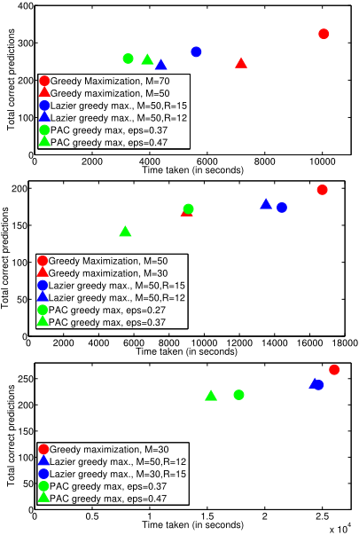
We conducted experiments with different values of n and k. As a baseline, we use greedy maximization and lazier greedy maximization. Since we cannot compute F exactly, greedy maximization simply uses an approximation, based on MLE estimates of conditional entropy, ignoring the resulting bias and making no attempt to reason about confidence bounds. Lazier greedy maximization, in each iteration, samples a subset of size R from X and selects from that subset the element that maximizes the estimated marginal gain. Neither greedy nor lazier greedy maximization employ lazy evaluations, i.e., pruning elements via a priority queue as in lazy greedy maximization, because the reliance on approximation of F means pruning is no longer justified. In addition, since lazy greedy maximization's pruning is based on marginal gain instead of F, the bias is exacerbated by the presence of two entropy approximation instead of one.

For greedy maximization and lazier greedy maximization, the number of samples M used to approximately compute F was varied from 10 to 100. For lazier greedy maximization, the value of R was also varied from 5 to 15. For PAC greedy maximization, the number of samples used to compute the upper and lower bounds were fixed to 20 and 10 respectively, while the parameter ✏1 was varied from 0.1 to 0.5. On average the length of each trajectory sampled was 30 timesteps and the experiments were performed on 30 trajectories for k = 1, 17 trajectories for k = 2 and 20 trajectories for k = 3, with 5 independent runs for k = 3 and 3 independent runs for k = 2 and k = 1. To avoid clutter, we show results for only the two best performing parameter settings of each algorithm.

Figure 1 shows the number of correct predictions (y-axis) against the runtime (x-axis) of each method at various settings of M, R and ✏. Thus, the top left is the most desirable region. In general, PAC greedy maximization performs nearly as well as the best-performing algorithm but does so at lower computational cost. Naively decreasing the number of samples only worsens performance and does not scale with k as the computational cost of even performing greedy maximization with nominal samples is huge in the bottom plot. PAC greedy maximization on the other hand performs well in all the three settings and scales much better as k increases, making it more suitable for real-world problems.

9 Conclusions &FutureWork

This paper proposed PAC greedy maximization, a new algorithm for maximizing a submodular function F when computing F exactly is prohibitively expensive. Our method assumes access to cheap confidence bounds on F and uses them to prune elements on each iteration. When F involves entropy, as is common in many applications, obtaining confidence bounds is complicated by the fact that no unbiased estimator of entropy exists. Therefore, we also proposed novel, cheap confidence bounds on conditional entropy that are suitable for use by PAC greedy maximization. We proved that the resulting method has bounded error with high probability. Our empirical results demonstrated that our approach performs comparably to greedy and lazier greedy maximization, but at a fraction of the computational cost, leading to much better scalability. In future work, we aim to develop good strategies for clustering observations to obtain tight upper confidence bounds on conditional entropy, and to combine our upper and lower confidence bounds with more sophisticated best-arm identification algorithm sto produce an even more efficient version of PAC greedy maximization.

Acknowledgments

We thank Henri Bouma and TNO for providing us with the dataset used in our experiments. We also thank the STW User Committee for its advice regarding active perception for multi-camera tracking systems. This research is supported by the Dutch Technology Foundation STW (project #12622), which is part of the Netherlands Organisation for Scientific Research (NWO), and which is partly funded by the Ministry of Economic Affairs. Frans Oliehoek is funded by NWO Innovational Research Incentives Scheme Veni #639.021.336.