Correlation Complexity of Classical Planning Domains

1 Introduction

Recently, potential heuristics [Pommerening et al., 2015] have been introduced as a new class of heuristics for classical planning. A potential heuristic is defined by specifying a numerical (possibly negative) weight for every fact of a planning task. The heuristic value of a state is then simply the sum of weights of the facts that are present in that state. Potential heuristics can be viewed as linear combinations of trivial indicator functions, where each indicator function tests whether a certain fact is present in the given state.

Due to their simple structure, potential heuristics can be evaluated very efficiently. Of course, the quality of their heuristic estimates critically depends on the choice of weights. In past work, finding suitable weights has been cast as an optimization problem with encouraging results [Pommerening et al., 2015; Seipp et al., 2015].

However, it is clear that for challenging planning tasks, such simple potential heuristics cannot be truly informative, as complex interactions between different state variables cannot be adequately captured. Fortunately, the idea can be readily generalized by considering indicator functions for more complex state features than individual facts. An obvious generalization is to test for the presence of a set (or conjunction) of facts, similar to the generalization from the hmax heuristic to Haslum and Geffner's hm heuristics [2000] or to the generalization from atomic to general projections in pattern database (PDB) heuristics [e.g., Edelkamp, 2001].

It is easy to see that with such a generalization, arbitrary heuristics can be expressed as potential heuristics: in the extreme case, we can introduce a separate feature for every single state s and set its weight to the actual cost-to-goal h⇤ (s)

of that state. Again, this is analogous to the hm heuristics, which converge to h⇤ as m increases to the number of facts of the planning task, and to PDB heuristics, which similarly converge to h⇤ as the set of pattern variables grows to include all variables. However, it is equally easy to see that in all three cases, the size of the representation explodes, and the heuristics become unmanageable on their way to perfection.

This raises the question how complex these heuristics need to become in order to faithfully capture the critical interactions between state variables. Many planning domains are known to admit polynomial domain-specific solution algorithms [e.g., Helmert, 2003]. Perhaps "simple" heuristics only considering conjunctions of 2 or 3 facts are already highly accurate in these "simple" domains?

Unfortunately, there is bad news in the literature: Helmert and Mattm¨uller [2008] showed that hm and (single) PDB heuristics based on conjunctions of bounded size give rise to arbitrarily bad heuristics in all domains they studied. However, they also showed that additive heuristics based on multiple PDBs can be significantly more accurate. This is not just good news for PDBs but also for potential heuristics, which are additive combinations of simpler heuristics by definition.

So just how complex does a potential heuristic have to be so that solving a planning task becomes simple? Following in Hoffmann's [2005] footsteps, we formalize this question by considering per-domain results for the state space topology of planning tasks. Hoffmann studied the search space topology of a fixed heuristic, namely the optimal delete relaxation heuristic h+. Delete relaxation heuristics are rarely perfect but frequently good: to quantify this, Hoffmann focused on the size of local minima in the state space to distinguish "easy" from "difficult" domains for h+.

In contrast, potential heuristics can be as accurate as we wish, at a cost in heuristic complexity. To reflect this degree of control, in our theoretical analysis we are more demanding with state space topology, looking for heuristics that exhibit no local minima at all. The question, then, is how complex - measured in the size of the conjunctions required - a potential heuristic needs to be in order to have no local minima. 1

In this paper, we study this complexity measure for a number of well-known planning domains. It turns out that the results are very encouraging, motivating further study of potential heuristics with conjunctive features. We believe that this outcome is also relevant to researchers with no particular interest in potential heuristics, or even heuristic search.

1 Throughout the paper, by "local minimum" we mean any state which does not have a successor with lower heuristic value. This includes states within heuristic plateaus.

At its core, the complexity measure we introduce describes how tightly interrelated different aspects of a planning task are, and to what extent these aspects can be considered separately. Within planning as heuristic search, such a measure is clearly relevant for approaches such as planning with pattern databases [Edelkamp, 2001; Haslum et al., 2007; Pommerening et al., 2013], critical-path heuristics [Haslum and Geffner, 2000; Haslum et al., 2005], semi-relaxed plan heuristics [Keyder et al., 2014], conjunctive landmarks [Keyder et al., 2010], or flow heuristics with merges [Bonet and van den Briel, 2014]. However, we think that such a measure of "interrelatedness" can be equally useful for non-heuristic planning approaches, such as factored planning [Brafman and Domshlak, 2013], planning with decision diagrams [e.g., Torralba, 2015], and compilations to SAT [e.g., Rintanen, 2012; Suda, 2014].

The general idea of measuring the degree of interrelatedness between state variables of a planning task is not new. In a line of research with very similar motivations to ours, Chen and Gim´enez [2007; 2009] studied several notions of width for planning tasks, where low width implies low complexity of planning. In the same spirit, Lipovetzky and Geffner [2012] also introduced a notion of width (different from those of Chen and Gim´enez) and exploited it to efficiently solve a large number of standard planning benchmarks. We return to this work towards the end of the paper, where we discuss the relationship between our complexity measure and the existing notions of width.

2 Planning Formalism

We consider SAS+ [B¨ackstr¨om and Nebel, 1995] planning tasks ⇧ = hV↪ O↪ sI↪ s?i, where V is a finite set of state variables, O is a finite set of operators, sI is the initial state, and s? is the goal.

Each state variable v 2 V has a finite domain dom(v). A pair hv↪ di with v 2 V and d 2 dom(v) is called a fact. A set of facts is consistent if all contained facts belong to different variables. A consistent set of facts p is called a partial variable assignment. We write vars(p) to denote the set of variables to which the facts in p belong. For v 2 vars(p) we write p[v] to denote the value d 2 dom(v) for which hv↪ di 2 p. If vars(p) = V, p is called a state.

The initial state sI is a state, and the goal s? is a partial variable assignment. A state s is consistent with partial variable assignment p if p ✓ s. A state s is a goal state if it is consistent with the goal s?. In some contexts, we refer to partial variable assignments as (state) features and say that a state has the feature F if it is consistent with F.

Each operator o 2 O is given as a pair o = hpre(o)↪ eff(o)i, where the precondition pre(o) and the effect eff(o) are partial variable assignments. Operator o is applicable in state s if s is consistent with pre(o). In this case, o may be applied in s, yielding the successor state sJoK defined by sJoK[v] =

eff(o)[v] for all v 2 vars(eff(o)) and sJoK[v] = s[v] for all other variables v. We write succ(s) for the set of all successor states of s, i.e., succ(s) = ¶sJoK ♣ o 2 O is applicable in s♦. Our focus in this paper is on planning algorithms that do not provide quality guarantees for the plans they find, and hence we do not consider operator costs.

For a state s, an s-plan ho1↪ ▷ ▷ ▷ ↪ oni is a finite sequence of operators such that sJo1KJo2K ▷ ▷ ▷ JonK is a goal state. We say that s is solvable if an s-plan exists and unsolvable otherwise. The task ⇧ is solvable if the initial state sI is solvable. A state s is reachable if hV↪O↪ sI↪ si is solvable. Finally, a heuristic is a function mapping states to Z [ ¶1♦.

3 Potential Heuristics

Potential heuristics were introduced by Pommerening et al. [2015] as linear combinations of indicator functions, where each indicator function tests if a given fact is contained in the evaluated state. We generalize the definition to allow conjunctive state features. Throughout the paper, we write indicator functions using Iverson brackets [Knuth, 1992].

Definition 1 (potential heuristic). Let ⇧ be a planning task,

let F be a set of state features of ⇧, and let w : F ! Z[¶1♦. The potential heuristic with features F and weight function

w is the function ' mapping each state s of ⇧ to the integer

Note that we limit the definition to integer or infinite weights because these are sufficient for our purposes and simplify presentation. In other contexts, it may be preferable to permit arbitrary real-valued weights.

We measure the level of complexity of a potential heuristic by the size of the largest conjunction it uses as a feature, which we call its dimension.

Definition 2 (dimension). A potential function with features F has dimension maxF2F ♣F ♣.

Rephrasing what we said earlier using this terminology, previous work introduced potential heuristics of dimension 1, while we consider arbitrary dimensions.

The dimension of a potential heuristic is not the only natural way to measure its complexity. Alternative, more finegrained measures include the number of features or the sum of features sizes. We choose to focus on the dimension because our results do not require more fine-grained measures and because dimension is a natural analogue to well-known parameters of other heuristics, such as the parameter m in the hm heuristics and the pattern size in PDB heuristics.

For tasks with n state variables, potential heuristics of dimension d can be evaluated in time O(nd ). In the common case where a family of planning tasks has a fixed bound on the number of effects in each operator, this can be improved to O(nd-1 ) with incremental computations, i.e., when asked to compute the heuristic value of a state given its parent state, generating operator and parent heuristic value. (To see this, note that if an operator changes k state variables, then only features involving at least one of these k state variables and hence at most d - 1 other state variables need to be considered. The total number of such features can be bounded by

2k · (n - k)d-1 , which is O(nd-1 ) for constant k.) In particular, in this case potential heuristics of dimension 1 can be incrementally computed in constant time and potential heuristics of dimension 2 can be incrementally computed in time O(n).

4 State Space Topology

We want to study potential heuristics without local minima. To formalize this, we must first clarify what we mean by having no local minima. A tentative definition might be: "every non-goal state has a successor with lower heuristic value". However, this is too strict: in a finite state space, such a definition implies that there is a strictly descending path towards a goal state from every state, which is impossible to satisfy if the task has any unsolvable states.

Hence, we only require that solvable states have successors with lower heuristic value. To avoid a heuristic search algorithm from getting trapped in an unsolvable region of the state space, we also require that unsolvable successors s0 of a solvable state s never have a lower heuristic value than s.

A second problem is that planning tasks often include "impossible" states that violate physical constraints, such as two blocks being stacked on top of each other in the Blocksworld domain. It would be unnecessarily restrictive to require that the state space topology is also well-behaved for such impossible states. However, there is in general no simple way to distinguish possible from impossible states without complicating the definition of planning tasks. A simple remedy is to restrict attention to reachable states.

Definition 3 (alive). A state is alive if it is solvable, reachable, and not a goal state.

We can now introduce two criteria that together imply absence of local minima.

Definition 4 (descending). A heuristic h is descending if all alive states have an improving successor. In symbols, for all states s:

Definition 5 (avoiding dead ends). A heuristic h avoids dead ends if all improving successors of alive states are solvable. In symbols, for all states s and s0 :

Given these two properties typical heuristic search algorithms for satisficing planning are guided directly towards the goal. We give a formal proof for simple hill-climbing (Algorithm 1).

Theorem 1. Let h be a descending, dead-end avoiding heuristic for a planning task ⇧. Let L = h(sI)-mins2S h(s), where S is the set of all states of ⇧.

Then simple hill-climbing with h solves ⇧ after at most L state expansions if ⇧ is solvable and returns with failure after at most L state expansions if ⇧ is unsolvable.

Proof: Consider the case where ⇧ is solvable. For the while loop, we show the loop invariant that s is reachable and solvable. Reachability is trivial. For solvability, s is initially solvable, and in every iteration of the loop, the chosen state s0 is Algorithm 1 Simple hill-climbing.

s sI ⇡ hi while s is no goal state do improvement false for s0 2 succ(s)↪ in any order do if h(s0 ) < h(s) then improvement true append o 2 O with sJoK = s0 to ⇡ s s0 break if improvement is false then fail return ⇡

solvable because s is alive (because it is not a goal state and due to the loop invariant, it is reachable and solvable), s0 is an improving successor of s and h avoids dead ends.

We next show that the algorithm terminates by returning a plan (rather than failing or not terminating). Because h is descending, an improving state is always found inside the for loop, so the while loop never fails. Moreover, the while loop must finish with a bounded number of iterations because h(s) decreases in every iteration and hence the sequence of expanded states never repeats. This proves that the algorithm terminates and also establishes the stated bound on L. (Note that h(s) is an integer and hence must decrease by at least 1 in every iteration.)

In the case where ⇧ is unsolvable, simple hill-climbing fails as soon as there is no more successor with lower heuristic value. As in the previous case, h(s) cannot decrease more than L times, bounding the number of steps. ⇤

The same result holds, with the same proof, for steepest ascent hill-climbing, a variant of hill-climbing that always moves to a successor s0 minimizing the h value.

In the case where ⇧ is solvable, the result also extends to the three most common satisficing planning algorithms: standard greedy best-first search a.k.a. eager greedy search [Russell and Norvig, 2003], greedy best-first search with deferred evaluation a.k.a. lazy greedy search [Richter and Helmert, 2009] and enforced hill-climbing [Hoffmann and Nebel, 2001]. To see this, observe that for descending, deadend avoiding heuristics applied to solvable planning tasks, eager search expands the same states as steepest ascent hillclimbing, enforced hill-climbing expands the same states as simple hill-climbing, and lazy search evaluates the same states as simple hill-climbing.

We conclude this section by looking in a bit more depth at the requirement of avoiding dead ends. A special case in which this property holds for all heuristics are tasks where no solvable states have unsolvable successors. Hoffmann [2005] calls such planning tasks harmless. A common special case of harmless planning tasks are undirected tasks, where s 2 succ(s0 ) iff s0 2 succ(s).

Instead of heuristics that avoid dead ends, one can make the stricter requirement of recognizing dead ends [Hoffmann, 2005], i.e., requiring h(s) = 1 for all unsolvable states. This stricter property is not needed for Theorem 1, but if it is given and the heuristic is known to be safe (i.e., h(s) = 1 guarantees that the state is unsolvable), then the equivalent of the theorem for enforced hill-climbing, eager greedy search and lazy greedy search also holds in the case of unsolvable planning tasks.

Instead of strengthening the requirement of avoiding dead ends, one could also consider the weaker requirement that unsolvable states are never among the best successors (minimizing h) of solvable states. This weaker requirement would still be sufficient for establishing a result like Theorem 1 for steepest ascent hill-climbing and eager greedy search, but not for simple or enforced hill-climbing or lazy greedy search.

5 Correlation Complexity

We now put the pieces of the previous two sections together: correlation complexity measures how complex a potential heuristic must be to obtain a favorable state space topology.

Definition 6 (correlation complexity of a planning task). The correlation complexity of a planning task ⇧ is the minimum dimension d of all descending, dead-end avoiding potential heuristics for ⇧.

The correlation complexity of a planning task is trivially bounded from above by the number of state variables n: in the worst case, we can define a feature with weight h⇤ (s) for every state s, and because ♣s♣ = n, such a potential heuristic has dimension n. In particular, this guarantees that the correlation complexity of planning tasks is well-defined.

The definition can be extended to planning domains, which for the purposes of this paper are simply (usually infinite) sets of planning tasks.

Definition 7 (correlation complexity of a planning domain). The correlation complexity of a planning domain is the maximal correlation complexity of all planning tasks in the domain, or 1 if no maximum exists.

If a domain has low correlation complexity, this is a sign that no complex interactions between variables need to be considered in order to solve planning tasks in this domain. Hence, low correlation complexity is an indication that a planning domain is "easy".

A formal tractability result for planning in such a domain does not immediately follow because Definition 7 does not guarantee that a low-dimension potential heuristic for a given planning task is easy to construct - it only guarantees that such a potential heuristic exists. Moreover, planning domains with low correlation complexity can have exponentially long plans. For example, it is easy to construct "binary counter" tasks (⇥i)i≥1 with correlation complexity 1 where ⇥i requires plans of length 2i to solve. In the absence of such complications, low correlation complexity indeed implies tractability.

Theorem 2. Let D be a planning domain with correlation complexity d < 1, and let p be a polynomial such that given ⇧ 2 D with encoding size n,

1. a descending, dead-end avoiding potential heuristic '⇧ of dimension d can be computed in time p(n), and
2. feature weights are polynomially bounded: ♣w(F)♣  p(n) for all features F of '⇧.

Then plan generation in D can be solved in polynomial time.

Proof: A task with encoding size n has at most n state variables, and hence '⇧ has no more than O(nd ) features. Together with the bound on the individual weights, it follows that ♣'⇧(s)♣  O(nd )p(n) for all states s, and hence the difference between the heuristic values of any two states is bounded by a polynomial in n.

The result follows with Theorem 1, as L is bounded by a polynomial in n, and each heuristic evaluation can be performed in time O(nd ), which is also polynomial in n. ⇤

6 Properties of Potential Heuristics

In the rest of the paper, we study the correlation complexity of some common planning domains. Towards this end, we first establish some general properties of potential heuristics, concluding in two criteria to show that a task has correlation complexity at least 2. We begin with a result that is related to the incremental computation of potential heuristics.

Theorem 3. Let ' be a potential heuristic for a planning task ⇧. Let s be a state of ⇧, let o be an operator applicable in s,

Proof: All other features are either present in both s and s0 or absent in both s and s0 . Their weights cancel out in the difference. ⇤

Consider a heuristic h and an operator o applicable in a state s. We say that o is good in s under h if h(sJoK) < h(s) and bad in s under h otherwise. We say that a planning task is in normal form if vars(eff(o)) ✓ vars(pre(o)) for all operators o [cf. Pommerening and Helmert, 2015]. It is easy to see that for tasks in normal form, whether or not an operator is good under a potential heuristic of dimension 1 does not depend on the state s: either o improves the heuristic value in all states where it is applicable, or it does so in no state. Hence, for potential heuristics of dimension 1 we can speak of good or bad operators without referring to a specific state.

We say that operator o is critical in planning task ⇧ if there exists an alive state s such that every s-plan includes o. (In other words, o is an action landmark in some alive state.)

Theorem 4. Let ' be a descending potential heuristic of dimension 1 for a planning task ⇧ in normal form.

If o is critical in ⇧, then o is good under '.

Proof: Because o is critical, there exists an alive state s from which every s-plan includes o. Because ' is descending, there exists a sequence of operator applications that reach a goal state from s and decrease the heuristic value in every step. All operators applied in this sequence must be good, and one of them must be o. ⇤

If o has an inverse operator o0 (i.e., sJoKJo0 K = s for some state s), then o and o0 cannot both be good: if going from s to sJoK decreases the heuristic value, then returning from sJoK to s by applying o0 must increase it to the original value. Together with Theorem 4 we obtain the first criterion for showing that a task cannot have correlation complexity 1.

Theorem 5. Let ⇧ be a planning task in normal form, and let o and o0 be critical operators of ⇧ that are inverses of each other. Then ⇧ has correlation complexity at least 2.

Proof: Assume the contrary: there exists a descending potential heuristic ' of dimension 1. From the previous theorem, o and o0 are both good under '. Inverse operators cannot both be good: a contradiction. ⇤

For the second criterion, we need the notion of dangerous operators. Operator o is dangerous in task ⇧ if there exists an

alive state s in which o is applicable and sJoK is unsolvable. Theorem 6. Let ⇧ be a planning task in normal form, and let o be an operator that is critical and dangerous in ⇧. Then ⇧ has correlation complexity at least 2.

Proof: Assume the contrary: there exists a descending potential heuristic ' of dimension 1 that avoids dead ends. Since o is critical, it is good under ' (Theorem 4). But o is also dangerous and hence leads from an alive to an unsolvable state. By the definition of avoiding dead ends, this means that o cannot be good: a contradiction. ⇤

7 Spanner

We now begin our case studies of planning domains. In the Spanner domain (IPC 2014), an agent has to walk to a gate along a chain of m locations l1-l2-▷ ▷ ▷ -lm, with the gate at lm. At the gate there are n nuts that the agent has to tighten with n single-use spanners that it must pick up along the way. The agent can only move towards the gate, not backwards.

Lemma 1. Spanner has correlation complexity at least 2.

Proof: Consider a task with two locations l1, l2 and one spanner at l1. Walking from l1 to l2 is critical, but dangerous. (Walking before picking up the spanner leads to an unsolvable state.) The result follows with Theorem 6. ⇤

Theorem 7. Spanner has correlation complexity 2.

Proof: Let ⇧ be a Spanner task with n spanners and m locations. For any location li let Si be the number of spanners at all locations lj with j < i. Walking to location li while carrying fewer than Si spanners leads to an unsolvable state.

The following weight function defines a descending, deadend avoiding potential heuristic ' of dimension 2 for ⇧. The result then follows with the preceding lemma.

We show that ' is descending and avoids dead ends by showing that the heuristic difference induced by picking up a spanner or tightening a nut is always negative and the potential difference induced by walking from li-1 to li is negative iff the agent is carrying Si spanners.

Picking up spanner j at location li changes the potential by m - i - m = -i < 0.

Tightening nut j is always done in location lm and changes the potential by -m - 1 - (-m) - (m - m) = -1.

Walking from li-1 to li while carrying s spanners changes the potential by Pik=1 (Sk - 1) - Pi-1 k=1 (Sk - 1) + s((m - i)-(m-(i-1))) = Si -s-1 which is negative iff s ≥ Si. ⇤

8 Gripper

In the Gripper domain (IPC 1998), a robot with two grippers has to move n balls from room A to room B. It can pick up and drop balls in either room and move between the two rooms. The robot always starts in room A and the goal is always to transport all balls to room B. In a SAS+ representation there is a variable specifying the position of the robot r 2 ¶A↪B♦ and variables for the position of each ball bi 2 ¶A↪ B↪ G1↪ G2♦ for 1  i  n. G1 and G2 stand for the two grippers.

Lemma 2. Gripper has correlation complexity at least 2.

Proof: In a Gripper task with more than 2 balls, moving from A to B and moving from B to A are both critical operators, and they are inverses of each other. The result follows with Theorem 5. ⇤

Theorem 8. Gripper has correlation complexity 2.

Proof: The following weight function defines a descending, dead-end avoiding potential heuristic of dimension 2 for the Gripper task with n balls. The result then follows with the preceding lemma.

The heuristic avoids dead ends because Gripper is undirected and hence harmless. To show that the heuristic is descending, we show by case distinction that every reachable non-goal state has an improving successor.

If the robot is in room A and can pick up a ball, picking it up changes the potential by -w(¶hbi↪Ai♦) + w(¶hbi↪Gji♦) = -8 + 4 = -4. If there is no ball to pick up, but the robot has g > 0 balls in its grippers, moving to room B changes the potential by w(¶hr↪Bi♦) - g · w(¶hr↪Bi↪ hbi↪Gji♦) = 1 - 2g < 0. If there are no balls to pick up and no balls in the grippers, the state is a goal state.

If the robot is in room B and has a ball in one of its grippers, dropping a ball changes the potential by -w(¶hbi↪ Gj i♦)-w(¶hr↪ Bi↪ hbi↪ Gj i♦) = -4-(-2) = -2. If it does not have a ball in its grippers, moving to room A changes the potential by -w(¶hr↪ Bi♦) = -1. ⇤

We remark that steepest ascent hill climbing with the given potential heuristic produces an optimal plan because picking up a ball in room A (improvement by 4) and dropping a ball in room B (improvement by 2) are always preferred to moving to the other room (improvement by 1).

9 VisitAll

In VisitAll (IPC 2011) an agent has to visit all vertices of a graph. In a SAS+ encoding of the tasks there is a Boolean variable for each vertex indicating whether the vertex has been visited and a variable storing the position of the agent.

VisitAll tasks are not in normal form but we can transform them to normal form by replacing each operator walk-A-B with two operators: one for the case where B is already visited and one to visit B for the first time. The transformed domain has the same states and successor state relation and hence has the same correlation complexity as the original one.

Lemma 3. VisitAll has correlation complexity at least 2.

Proof: Consider a task with a chain of four locations (l1-l2l3-l4) and initial location l2. Consider the following two alive states s and s0 : in both states, l2 and l3 are the locations that have already been visited. In s, the agent is at l2. In s0 , it is at l3. From s, we see that walk-to-visited-l2-l3 is critical; from s0 , we see that its inverse walk-to-visited-l3-l2 is critical. The result follows with Theorem 5. ⇤

Theorem 9. VisitAll has correlation complexity 2.

Proof: Let ⇧ be a task with n locations l1↪ ▷ ▷ ▷ ↪ ln forming a connected graph. (If the graph is unconnected, the task is unsolvable.) Let d(i↪ j) be the shortest path distance between li and lj . The following weight function defines a descending, dead-end avoiding potential function of dimension 2 for ⇧:

The result then follows with the preceding lemma.

The function avoids dead ends because VisitAll is harmless. To show that it is descending, we consider a non-goal state where the unvisited location with the highest index is lm. Moving one step in the direction of lm decreases the potential by at least 2m - P1i<m 2i = 2. ⇤

We remark that even though the construction uses exponential weights, it leads to a polynomial planning algorithm because singly exponential numbers require only linear space to represent (hence computing the heuristic is not expensive), and the length of the generated plan is at worst quadratic in the number of locations. (It never takes more than n steps to reach another previously unvisited location.)

10 Blocksworld

In Blocksworld [e.g., Slaney and Thi´ebaux, 2001] there are stacks of n blocks that must be rearranged from an initial to a goal configuration. We assume the following standard SAS+ encoding for the domain formulation without an explicit hand: for each block A there is a Boolean variable clear-A denoting whether another block can be stacked on top of A and a variable pos-A that specifies what is below A. The possible values of pos-A are one value B for each other block B and the special value T for being on the table. Operators move a clear block from one block onto another, from a block onto the table, or from the table onto a block.

Lemma 4. Blocksworld has correlation complexity at least 2.

Proof: Consider a task with initial state A-B-D-C (A is on top of the tower) and goal A-B-C-D. Moving A from B to the table and its inverse are critical. We apply Theorem 5. ⇤

Theorem 10. Blocksworld has correlation complexity 2.

Proof: Let ⇧ be a Blocksworld task with blocks B where sG is a goal state. We call the position of any block A in sG its target position GA (which may be the table). If a block is in its target position, it is correctly placed, otherwise misplaced. For each tower in sG, we number the blocks from top to bottom, i.e., the top block B of each tower has level(B) = 1, the block directly below it has level 2, etc. We call a block B controlled by a block A if B is anywhere below A in a tower of sG. We say a block is done in a state if it and all blocks that are below it in sG are correctly placed.

Blocksworld is undirected, and hence avoiding dead ends is trivial. The following weight function defines a descending potential heuristic of dimension 2 for ⇧. The result then follows with the preceding lemma.

Atomic features for all blocks A 2 B:

Conjunctive features for all blocks A↪B 2 B where B is controlled by A and all X 2 dom(pos-B) with X 6= GB:

In words, the conjunctive features punish situations where block A is correctly placed while block B controlled by A is misplaced. We now show that every reachable non-goal state s has an improving successor s0 .

If all not-done blocks are on the table in s, consider a notdone block A where GA is done. Moving A onto GA reduces the heuristic value by w(¶hpos-A↪ T i♦) = 1.

Otherwise, s has a tower of at least two blocks such that the top block A is not done. Let B denote the block below A. Consider state s0 reached by moving A onto the table.

If A is misplaced in s, then the atomic features change the heuristic value by w(¶hpos-A↪ T i♦) - w(¶hpos-A↪ Bi♦) in s0 , which is -1 or -3 and hence an improvement. The conjunctive features can only change if A is correctly placed in s0 , which implies GA = T. Then A controls no other blocks, and hence no conjunctive feature becomes true. Conjunctive features related to blocks controlling A may become false, but this only improves the heuristic value further.

If A is correctly placed in s, the part of the heuristic value that is due to atomic features increases by 1 when going from s to s0 . The change from conjunctive features is

A controls at least one misplaced block D because A is not done in s, and hence the right sum is at least 2level(A) . The left sum is at most Plevel(A)-1 i=1 2i = 2level(A) - 2, where the maximum is attained if all blocks controlling A are correctly placed in s. We get ∆  (2level(A) -2)-2level(A) = -2. This compensates the increase of 1 from the atomic features: s0 is an improving successor. This completes the proof. ⇤

Similar to VisitAll, the potential heuristics give rise to a polynomial planning algorithm despite the exponential weights. It is easy to verify that hill-climbing with these potential heuristics moves each block at most two times (steepest ascent hill-climbing) or three times (simple hill-climbing).

11 Tasks with Higher Correlation Complexity

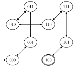
All the domains we studied so far have correlation complexity 2. The natural question is whether there are tasks with higher correlation complexity. We now answer this question in the affirmative by giving an example of a planning task with correlation complexity 3. The state space of the example task is shown in Figure 1. We obtained this task by mimicking the construction of the reflected binary code, also known as Gray code [Gray, 1953]. Gray code is based on nested layers of reflections, and because of these reflections, intuitively speaking, the state changes that need to be made in the example task in one half of the state space are exactly the opposite of the state changes that need to be made in the other half. This makes the "correct" operator to take heavily dependent on context and hence potential heuristics of low dimension cannot give sufficient guidance for this task.

Lemma 5. The planning task in Figure 1 has correlation complexity at least 3.

Proof: Any descending potential function for the task has to strictly decrease along the (unique) optimal plan. As the heuristic values are linear combinations of weights, each step in the plan yields a linear constraint over weights that is a necessary condition for a given potential function to be descending. For example, for the first step, we get the constraint

w0?? + w?0? + w??0 + w00? + w0?0 + w?00 > w0?? + w?0? + w??1 + w00? + w0?1 + w?01▷

Here, w0?? denotes the weight for the feature ¶hv1↪ 0i♦, w0?1 denotes the weight for the feature ¶hv1↪ 0i↪ hv3↪ 1i♦, etc.

Using basic algebra or a solver for linear programs, we can verify that there is no solution that satisfies all constraints. ⇤

Intuitively, the reason why potential heuristics of dimension 2 are not sufficient for the example is that one has to consider the values of both v1 and v2 to decide whether v3 should be changed from 0 to 1 to advance towards the goal, or whether the opposite transition is needed. Moreover, this dependency on v1 and v2 cannot be expressed by linear combinations of v1 and v2 because the correct decision is governed by their exclusive-or combination, v1 ⊕ v2.

Theorem 11. The planning task in Figure 1 has correlation complexity 3.

Proof: As mentioned in Section 5, the correlation complexity of a planning task is bounded from above by the number of state variables in the task. The result then follows with the preceding lemma. ⇤

This result concludes our case studies. In the following sections, we compare correlation complexity to related concepts from the literature.

12 Relation to Persistent HammingWidth

Chen and Gim´enez [2007] introduced four related concepts for measuring the width of a planning task. Width is an indicator of complexity: they describe a planning algorithm that finds solutions for solvable planning tasks in time that scales exponentially (only) in the width of the task.

The most general of the width concepts considered by Chen and Gim´enez is persistent Hamming width. A planning task has persistent Hamming width k if it is unsolvable, or if from every reachable non-goal state s, it is possible to reach a state s0 where the set of satisfied goals in s0 is a strict superset of the set of satisfied goals in s, and none of the states on the path from s to s0 differs from s in more than k state variables.

Unlike correlation complexity, which is defined for all planning tasks, persistent Hamming width is undefined for solvable planning tasks where an unsolvable state can be reached. The planning algorithm described by Chen and Gim´enez is incomplete when applied to such tasks. However, for planning domains with bounded width, it is a complete polynomial-time planning algorithm.

The work by Chen and Gim´enez resembles the state space topology study of Hoffmann [2005] in the sense that it measures how much work a search algorithm must perform to compensate for inaccuracies of a heuristic. (Even though Chen and Gim´enez do not explicitly consider heuristics, their search algorithm behaves similarly to enforced hill-climbing using a heuristic counting the number of unsatisfied goals.) In contrast, correlation complexity measures how complex a heuristic must be in order to guide a search algorithm directly to the goal. As the main purpose of the search component in a heuristic search algorithm is to compensate for inaccuracies of the heuristic, needing more complex heuristics vs. needing more search can be viewed as two faces of the same coin.

It is not hard to find examples where correlation complexity and persistent Hamming width widely disagree on the "difficulty" of a planning domain. This is to be expected: in both cases, the intuition is that low complexity means that solutions can be found efficiently (in the case of correlation complexity with the added difficulty that low complexity only means that accurate potential heuristics of low dimension exist, but does not tell us how to construct them). The converse is not necessarily true: if a domain has high persistent Hamming width (for example), this does not imply that planning is hard in this domain, only that the particular algorithm considered by Chen and Gim´enez might not be suitable for it.

A simple example of disagreement between the two measures are domains with reachable dead ends, like the Spanner domain (Section 7). It has correlation complexity 2, but no well-defined persistent Hamming width. On tasks with more than one spanner, the algorithm by Chen and Gim´enez will fail because it tries to achieve one of the goals as quickly as possible, which means picking up only one spanner and reaching a dead end.

The two measures can also disagree in domains without dead ends. As an example, consider a family of planning tasks where the n-th task encodes an n-ary binary counter counting backwards. We can encode this task with n state variables ¶vn-1↪ ▷ ▷ ▷ ↪ v0♦, all with domain ¶0↪ 1♦, set to 1 initially and required to be 0 in the goal. The state ¶hvn-1↪ dn-1i↪ ▷ ▷ ▷ ↪ hv0↪ d0i♦ represents the counter value Pn-1 i=0 di2i , and there are n operators that encode decrementing the counter by 1. (Each operator encodes one of the cases of 0, . . . , n-1 carries.)

The correlation complexity for all these tasks is 1: using weight 2i for the feature ¶hvi↪ 1i♦ results in the perfect heuristic. The persistent Hamming width of the n-th task is n: from the state representing the counter value 2n-1 , all n state variables must be changed to make progress towards the goal.

In a later paper, Chen and Gim´enez [2009] generalized persistent Hamming width to macro persistent Hamming width, which additionally allows the use of macros computed on the fly that temporarily pass through states whose Hamming distance from the current state is larger than k. This modification leads to tractability results for some domains where no such results could be obtained for persistent Hamming width, such as a formulation of Blocksworld with an explicit arm. However, adding macros does not influence the overall greediness of the approach (trying to achieve each individual goal as quickly as possible), and hence the modified algorithm still gets trapped in dead ends in the Spanner domain. It also does not improve over persistent Hamming width in the binary counter domain, although it does lead to tractability in a formulation of Towers of Hanoi, where it generates (compact representations of) exponentially long plans in polynomial time [Chen and Gim´enez, 2009].

13 Relation to Serialized IteratedWidth

Lipovetzky and Geffner [2012; 2014] also introduced a notion of width for planning tasks. Very roughly speaking, according to their definition a planning task has width k if interactions between at most k facts must be considered in order to solve a planning task. Lipovetzky and Geffner observe that optimal solutions to a planning task can be found in time that is only exponential in the width of the task.

Most of the commonly considered planning domains do not admit polynomial-time optimal planning algorithms unless P = NP [Helmert, 2003], and consequently most planning domains do not have bounded width. To the best of our knowledge, no examples of planning domains with bounded width have been described in the literature. However, Lipovetzky and Geffner observe that many common benchmark domains have bounded width when restricted to the case where the goal is a single fact, and that many of them can be solved by serialization, focusing on one goal fact at a time. (This does not contradict the previously mentioned complexity result because such serialized solutions are not necessarily optimal, even if the plans for the individual goal facts are.) Based on this observation, they introduce the Serialized Iterated Width algorithm, which achieves polynomial runtime on a wide range of benchmark domains.

This notion of width and the Serialized Iterated Width algorithm do not give rise to polynomial algorithms in cases like the Spanner domain (Section 7) that require global resource reasoning. Spanner tasks with n spanners have width ⇥(n) and cannot be serialized in the sense of Lipovetzky and Geffner, as focusing on one subgoal at a time and solving it optimally necessarily leads to a dead end. Similarly, the binary counter example from the previous section requires unbounded width to be solved with the Serialized Iterative Width algorithm: this is generally true for planning tasks where an exponential number of steps can be required to achieve the next goal fact. These are examples of domains with bounded correlation complexity but unbounded width.

However, it is also possible to construct tasks with low width and high correlation complexity. Given any planning task with correlation complexity n, we can create a new task (not equivalent to the original one) with width 1 by performing the usual conversion to a single goal fact (adding an artificial goal fact that can be achieved once the actual goal has been reached) and then adding a "cheating" operator that is only applicable in the initial state and directly achieves the artificial goal. The resulting task can be solved by a plan consisting only of the cheating operator and has width 1. However, it still has correlation complexity n because correlation complexity considers all alive states, and hence having one obvious short solution does not automatically lead to low correlation complexity.

14 Conclusion

We introduced a new measure for the complexity of classical planning tasks. Correlation complexity measures how complex the features of a potential heuristic must be for the induced state space to contain no local minima.

Correlation complexity is a way to quantify how interrelated the state variables of a task are. Planning tasks for which it is necessary to take into account large conjunctions of facts have high correlation complexity. The benchmark planning domains we studied in this paper all have a low correlation complexity of 2. Given that potential heuristics with low dimension can be evaluated very efficiently, our results motivate further research on how to find good features and weights for potential heuristics automatically.

We also described an artificial planning task with correlation complexity 3, but so far we have no examples of "naturally occurring" planning domains that are tractable, yet have high correlation complexity. We believe that studying correlation complexity in a wider set of benchmark domains could be useful to further improve our understanding of what makes planning hard and what makes easy planning tasks easy.

Acknowledgments

This work was supported by the Swiss National Science Foundation (SNSF) as part of the project "Reasoning about Plans and Heuristics for Planning and Combinatorial Search" (RAPAHPACS).