
Goal Recognition Design with Stochastic Agent Action Outcomes
Proceedings of the Twenty-Fifth International Joint Conference on Artificial Intelligence. Pages 3279-3284.
Abstract
Goal Recognition Design (GRD) problems involve identifying the best ways to modify the underlying environment that the agents operate in, typically by making a subset of feasible actions infeasible, in such a way that agents are forced to reveal their goals as early as possible. Thus far, existing work assumes that the outcomes of the actions of the agents are deterministic, which might be unrealistic in real-world problems. For example, wheel slippage in robots cause the outcomes of their movements to be stochastic. In this paper, we generalize the GRD problem to Stochastic GRD (S-GRD) problems, which handle stochastic action outcomes. We also generalize the worst-case distinctiveness (wcd) measure, which measures the goodness of a solution, to take stochasticity into account. Finally, we introduce Markov decision process (MDP) based algorithms to compute the wcd and minimize it by making up to k actions infeasible.
- [Bellman, 1957] Richard Bellman. Dynamic Programming. Princeton University Press, 1957.
- [Geffner and Bonet, 2013] Hector Geffner and Blai Bonet. A Concise Introduction to Models and Methods for Auto- mated Planning. Morgan & Claypool Publishers, 2013.
- [Geib and Steedman, 2007] Christopher Geib and Mark Steedman. On natural language processing and plan recognition. In Proceedings of the International Joint Conference on Artificial Intelligence (IJCAI), pages 1612-1617, 2007. IJCAI
- [Jarvis et al., 2005] Peter Jarvis, Teresa Lunt, and Karen My- ers. Identifying terrorist activity with AI plan recognition technology. AI Magazine, 26(3):73-81, 2005.
- [Johnson, 2010] W. Lewis Johnson. Serious use of a serious game for language learning. International Journal of Arti- ficial Intelligence in Education, 20(2):175-195, 2010.
- [Kelley et al., 2012] Richard Kelley, Liesl Wigand, Brian Hamilton, Katie Browne, Monica Nicolescu, and Mircea Nicolescu. Deep networks for predicting human intent with respect to objects. In Proceedings of the International Con- ference on Human-Robot Interaction (HRI), pages 171- 172, 2012.
- [Keren et al., 2014] Sarah Keren, Avigdor Gal, and Erez Karpas. Goal recognition design. In Proceedings of the International Conference on Automated Planning and Scheduling (ICAPS), pages 154-162, 2014.
- [Keren et al., 2015] Sarah Keren, Avigdor Gal, and Erez Karpas. Goal recognition design for non-optimal agents. In Proceedings of the AAAI Conference on Artificial Intel- ligence (AAAI), pages 3298-3304, 2015.
- [Keren et al., 2016a] Sarah Keren, Avigdor Gal, and Erez Karpas. Goal recognition design with non-observable ac- tions. In Proceedings of the AAAI Conference on Artificial Intelligence (AAAI), 2016.
- [Keren et al., 2016b] Sarah Keren, Avigdor Gal, and Erez Karpas. Privacy preserving plans in partially observable environments. In Proceedings of the International Joint Conference on Artificial Intelligence (IJCAI), 2016. IJCAI
- [Kolobov, 2013] Andrey Kolobov. Scalable Methods and Ex- pressive Models for Planning Under Uncertainty. PhD the- sis, University of Washington, 2013.
- [Lee et al., 2012] Seung Lee, Bradford Mott, and James Lester. Real-time narrative-centered tutorial planning for story-based learning. In Proceedings of the International Conference on Intelligent Tutoring Systems (ITS), pages 476-481, 2012.
- [Mausam and Kolobov, 2012] Mausam and Andrey Kolobov. Planning with Markov Decision Processes: An AI Perspec- tive. Synthesis Lectures on Artificial Intelligence and Ma- chine Learning. Morgan & Claypool Publishers, 2012.
- [McQuiggan et al., 2008] Scott McQuiggan, Jonathan Rowe, Sunyoung Lee, and James Lester. Story-based learning: The impact of narrative on learning experiences and out- comes. In Proceedings of the International Conference on Intelligent Tutoring Systems (ITS), pages 530-539, 2008.
- [Min et al., 2014] Wookhee Min, Eunyoung Ha, Jonathan Rowe, Bradford Mott, and James Lester. Deep learning- based goal recognition in open-ended digital games. In Proceedings of the AAAI Conference on Artificial Intel- ligence and Interactive Digital Entertainment (AIIDE), 2014.
- [Oh et al., 2010] Jean Oh, Felipe Meneguzzi, Katia Sycara, and Timothy Norman. ANTIPA: An agent architecture for intelligent information assistance. In Proceedings of the European Conference on Artificial Intelligence (ECAI), pages 1055-1056, 2010.
- [Oh et al., 2011a] Jean Oh, Felipe Meneguzzi, Katia Sycara, and Timothy Norman. An agent architecture for prognostic reasoning assistance. In Proceedings of the International Joint Conference on Artificial Intelligence (IJCAI), pages 2513-2518, 2011. IJCAI
- [Oh et al., 2011b] Jean Oh, Felipe Meneguzzi, Katia Sycara, and Timothy Norman. Probabilistic plan recognition for intelligent information agents: Towards proactive software assistant agents. In Proceedings of the International Con- ference on Agents and Artificial Intelligence (ICAART), pages 281-287, 2011.
- [Ramírez and Geffner, 2009] Miquel Ramírez and Hector Geffner. Plan recognition as planning. In Proceedings of the International Joint Conference on Artificial Intelligence (IJCAI), pages 1778-1783, 2009. IJCAI
- [Ramírez and Geffner, 2010] Miquel Ramírez and Hector Geffner. Probabilistic plan recognition using off-the-shelf classical planners. In Proceedings of the AAAI Conference on Artificial Intelligence (AAAI), 2010.
- [Ramírez and Geffner, 2011] Miquel Ramírez and Hector Geffner. Goal recognition over POMDPs: Inferring the in- tention of a POMDP agent. In Proceedings of the Interna- tional Joint Conference on Artificial Intelligence (IJCAI), pages 2009-2014, 2011. IJCAI
- [Son et al., 2016] Tran Cao Son, Orkunt Sabuncu, Christian Schulz-Hanke, Torsten Schaub, and William Yeoh. Solving goal recognition design using ASP. In Proceedings of the AAAI Conference on Artificial Intelligence (AAAI), 2016.
- [Tavakkoli et al., 2007] Alireza Tavakkoli, Richard Kelley, Christopher King, Mircea Nicolescu, Monica Nicolescu, and George Bebis. A vision-based architecture for intent recognition. In Proceedings of the International Sympo- sium on Advances in Visual Computing, pages 173-182, 2007.
- [Vilain, 1990] Marc Vilain. Getting serious about parsing plans: A grammatical analysis of plan recognition. In Pro- ceedings of the National Conference on Artificial Intelli- gence (AAAI), pages 190-197, 1990.
References were extracted automatically from the PDF and may contain errors.
Full text extracted automatically from the PDF; figures, tables and equations may differ. The PDF is the version of record.
1 Introduction
Plan and goal recognition problems aim to identify the actual plan or goal of an agent given its behavior. Within the last decade, researchers have made significant progress through synergistic integrations of techniques ranging from natural language processing [Vilain, 1990; Geib and Steedman, 2007] to classical planning [Ram´ırez and Geffner, 2009; 2010; 2011]. Plan and goal recognition problems have been used to model a number of applications ranging from software personal assistants and robots that anticipate the needs of the humans [Oh et al., 2010; 2011a; 2011b; Tavakkoli et al., 2007; Kelley et al., 2012]; intelligent tutoring systems that recognize sources of confusion or misunderstanding in students through their interactions with the system [McQuiggan et al., 2008; Johnson, 2010; Lee et al., 2012; Min et al., 2014]; and security applications that recognize terrorists plans [Jarvis et al., 2005].
The existing research in this area primarily focuses on developing better and more efficient techniques to recognize the plan or the goal of the user given a sequence of observations of the user's actions. For example, imagine a simplistic security example shown in Figure 1(a), where an agent (e.g., a potential terrorist) is at E3, it can move in any of the four cardinal directions, and its goal is one of three possible goals G1 (at B1), G2 (at A5), and G3 (at C5). Additionally, assume that it will move along a shortest path to its goal. Then, if it moves left to E2, we can deduce that its goal is G1. Similarly, if it moves right to E4, then its goal is either G2 or G3. However, if it is moves up to D3, we cannot make any informed deductions. In fact, if the agent moves along any one of its shortest paths to goal G3, throughout its entire path, which is of length 4, we cannot deduce whether its goal is either G2 or G3! This example illustrates one of the challenges with this approach, that is, there are often a large number of ambiguous observations that can be a result of a large number of goals. As such, it is difficult to uniquely determine the goal of the agent until a long sequence of actions is observed.
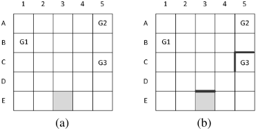
Therefore, Keren et al. [2014] very recently proposed an orthogonal approach to modify the underlying environment of the agent, in such a way that the agent is forced to reveal its goal as early as possible. They call this problem the Goal Recognition Design (GRD) problem. For example, if we block the actions (E3↪ up)↪ (C4↪ right)↪ (C5↪ up) in our example problem, where we use tuples (s↪ a) to denote that action a is blocked from cell s, then the agent can make at most 2 actions (i.e., right to E4 then up to D4) before its goal is conclusively revealed. Figure 1(b) shows the blocked actions. This problem finds itself relevant in many of the same applications of goal recognition because, typically, the underlying environment can be easily modified.
Keren et al. [2014] introduced the notion of worst-case distinctiveness (wcd), as a goodness measure that assesses the ease of performing goal recognition within an environment. The wcd of a problem is the longest sequence of actions an agent can take without revealing its goal. The objective in a GRD problem is then to find a subset of feasible actions to make infeasible such that the resulting wcd is minimized. In this problem, they make three assumptions: (i) the agents in the system will act optimally (i.e., agents will move along a shortest path to its goal); (ii) the outcomes of the actions of agents are deterministic; and (iii) the environment is fully observable (e.g., the outcomes of the actions can be observed). Since then, they have relaxed some of the assumptions [Keren et al., 2015; 2016a; 2016b]. Additionally, researchers have also addressed the original GRD problem using ASP [Son et al., 2016].
In this paper, we make two extensions to the GRD problem. The first extension limits the maximum number of feasible actions to make infeasible to k, which is a user-defined parameter. This extension is identical to the original problem if k = 1. The second extension relaxes the second assumption, that is, we assume that the actions of agents can be stochastic. Our approach lies in the use of Markov decision processes (MDPs) [Mausam and Kolobov, 2012] to formulate the planning problem of the agents within the GRD problem. Our choice is motivated by the fact that MDPs are often de facto models for representing planning problems with uncertainties. Finally, we also introduce new optimization methods that can be used to speed up the search.
2 Background
2.1 Classical Planning
A classical planning model [Geffner and Bonet, 2013], can be represented as a tuple hS↪ s0↪ A↪ f↪ C↪ Gi, where S is a finite and discrete state space; s0 is the start state of the agent; A is the set of actions, and A(s) ✓ A is the set of actions applicable in each state s 2 S; f : S ⇥A ! S is a deterministic state transition function, where s0 = f(s↪ a) is the successor state after applying action a 2 A(s) in state s; C : A ! R+ defines the cost for each action; and G is a set of goal states. A plan ⇡ = ha1↪ ▷ ▷ ▷ ↪ ani is a sequence of applicable actions that brings an agent from the starting state s0 to a goal state g 2 G. The cost of a plan C(⇡) = Pi C(ai) is the sum of the cost of each individual action in the plan. The goal is typically to find a cost-minimal plan ⇡⇤ = argmin⇡ C(⇡).
2.2 Goal Recognition Design (GRD)
A Goal Recognition Design (GRD) problem [Keren et al., 2014] is represented as a tuple P = hD↪Gi, where D = hS↪ s0↪A↪ f↪Ci captures the domain information and G is a set of possible goal states of the agent. The elements in the tuple D are as they are described in classical planning except that all actions have the same cost of 1. The worst case distinctiveness (wcd) of problem P is the length of a longest sequence of actions ⇡ = ha1↪ ▷ ▷ ▷ ↪ aki that is the prefix in cost-minimal plans ⇡⇤
g1 and ⇡⇤ g2 to distinct goals g1↪ g2 2 G Using our example problem of Figure 1(a), a longest sequence of actions that can lead to two distinct goals is h(E3↪ up)↪ (D3↪ up)↪ (C3↪ right)↪ (C4↪ right)i, where we use tuples (s↪ a) to denote that action a is taken from cell s. This sequence of actions can lead to either goals G2 or G3 and is of length 4. Thus, the wcd of the problem is 4.
The objective in GRD is to find a subset of actions ˆA⇤ ⇢ A such that if they are removed from the set of actions A, then the wcd of the resulting problem is minimized. This optimization problem is subject to the requirement that the cost of cost-minimal plans to achieve each goal g 2 G is the same before and after removing the subset of actions. More specifically, the objective is to find:
where ˆ P = h ˆD↪Gi is the problem with the resulting domain ˆD = hS↪ s0↪A ∩ ˆA↪ f↪Ci after removing actions ˆA, ⇡⇤ g is a cost-minimal plan to achieve goal g in the original problem P, and ˆ⇡⇤ g is a cost-minimal plan to achieve goal g in problem ˆ P. For example, blocking the actions (E3↪ up)↪ (C4↪ right)↪ (C5↪ up) in our example problem, where we use tuples (s↪ a) to denote that action a is blocked from cell s, will reduce the wcd of the problem to 2. Figure 1(b) shows the actions blocked. Then, the longest sequence of actions is h(E3↪ right)↪ (E4↪ up)i, which can lead to goals G2 or G3. Thus, the resulting wcd is 2.
2.3 Markov Decision Process (MDP)
A Stochastic Shortest Path Markov Decision Process (SSPMDP) [Mausam and Kolobov, 2012] is represented as a tuple hS↪ s0↪A↪T↪C↪Gi. It consists of a set of states S; a start state s0 2 S; a set of actions A; a transition function T : S ⇥ A ⇥ S ! [0↪ 1] that gives the probability T (s↪ a↪ s0 ) of transitioning from state s to s0 when action a is executed; a cost function C : S ⇥ A ⇥ S ! R+ that gives the cost C(s↪ a↪ s0 ) of executing action a in state s and arriving in state s0 ; and a set of goal states G ✓ S. The goal states are terminal, that is, T(g↪ a↪ g) = 1 and C(g↪ a↪ g) = 0 for all goal states g 2 G and actions a 2 A.
An SSP-MDP must also satisfy the following two conditions: (1) There must exist a proper policy, which is a mapping from states to actions with which an agent can reach a goal state from any state with probability 1. (2) Every improper policy must incur an accumulated cost of 1 from all states from which it cannot reach the goal with probability 1. In this paper, we will focus on SSP-MDPs and will thus use the termMDPs to refer to SSP-MDPs.
A "solution" to an MDP is a policy ⇡, which maps states to actions. Solving an MDP is to find an optimal policy, that is, a policy with the smallest expected cost. Value Iteration (VI) [Bellman, 1957] is one of the fundamental algorithms to find an optimal policy. It uses a value function V to represent expected costs. The expected cost of an optimal policy ⇡⇤ for the starting state s0 2 S is the expected cost V (s0), and the expected cost V (s) for all states s 2 S is calculated using the Bellman equation [Bellman, 1957]:
The action chosen by the policy for each state s is then the one that minimizes V (s).
3 Stochastic GRD Problem
We now describe the Stochastic GRD (S-GRD) problem, which is an extension of the original GRD problem along two dimensions. First, it limits the maximum number of actions to make infeasible to a user-defined parameter k. Second, it handles uncertainty in the actions of agents. In other words, an agent executing an action can now transition to multiple possible successor states with some probability. This extension is important because it can better model some real-world applications. For example, assume that the agent in our example in Figure 1 is a robot. Then, due to slippage, the robot has a small probability of staying where it is when it attempts to move. This characteristic, which cannot be captured by the original GRD problem, is captured in the S-GRD problem.
An S-GRD problem is also represented as a tuple P = hD↪Gi similar to GRD problems, except that the domain information D = hS↪ s0↪A↪T↪Ci is now represented similar to an MDP instead of a classical planning problem. Therefore, the elements in the tuple D are as they are described in MDPs. Like in the original GRD problem, we also assume here that all actions have the same cost of 1 though our model can be generalized to handle non-uniform costs.
Definition 1 (policy prefix) A policy prefix is a mapping ⇡ : S⇡ ! A, where s0 2 S⇡ ✓ S and, for each s 2 S⇡ ∩ ¶s0♦, there exists a state sequence hs0↪ s1↪ ▷ ▷ ▷ ↪ sn = si, where T (si↪ ⇡(si)↪ si+1) > 0 ^ si 2 S⇡.
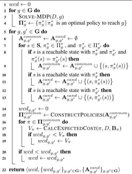
In other words, a policy prefix is a policy defined only on some states that are reachable from the start state s0. Figures 3(a) and 3(b) show examples of policy prefixes for an optimal policy to reach goal G2.
Definition 2 (boundary states) Given a policy prefix ⇡ : S⇡ !A, the set of boundary states B⇡ is defined as:
In other words, the set of boundary states is composed of all states s that are undefined in the policy prefix and whose predecessor state s0 is defined in the policy prefix.
Definition 3 (non-distinctive policy prefix) Given a problem P = hD↪Gi, a policy prefix ⇡ is a non-distinctive policy prefix in P if 9g0 ↪ g00 2 G such that g0 6= g00 and ⇡(s) = ⇡⇤ g0(s) = ⇡⇤ g00(s) for all states s 2 S⇡, where ⇡⇤ g0 and ⇡⇤ g00 are optimal policies for the problems hD↪ g0 i and hD↪ g00 i, respectively, and the goals g0 and g00 are terminal states. Otherwise, ⇡ is distinctive.
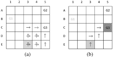
Intuitively, as long as an agent executes a non-distinctive policy prefix ⇡, it does not reveal its goal. However, the agent might eventually transition to a boundary state b 2 B⇡. If it transitions to goal boundary state b 2 G and stops executing any actions, then it has revealed its goal to be state b. If it transitions to a non-goal boundary state b ◁2 G and executes a particular action in that state, it might have revealed that its goal is not one of the two goals that define policy prefix ⇡ in Definition 3. For instance, consider distinct goals G2 and G3 in the example problem given in Figure 1. If the actions can either succeed with probability p or have no effect with probability 1-p, then Figure 2(a) shows the set of actions (denoted by arrows) that form all possible non-distinctive policy prefixes to those two goals and Figure 2(b) shows an example of one non-distinctive policy prefix and the corresponding set of boundary states (cells shaded in dark grey). In this case, there is only one boundary state for this policy prefix.
We now need a metric to assess the largest number of actions an agent can take or, equivalently, the largest cost an agent can incur before revealing its goal. Since transitions are stochastic, the number of actions or, equivalently, the cost incurred can be measured either in in the worst-case maximum or in the expectation. The worst-case maximum may be infinite (e.g., when the agent can transition back to its previous state and, thus, potentially get stuck in a loop), which prohibits meaningful comparisons. Therefore, in this paper, we choose to measure in the expectation and use the worstcase distinctiveness (wcd) as this measure.
Before defining the wcd, let V⇡(s0) denote the expected cost of reaching a boundary state b 2 B⇡ from the start state with policy prefix ⇡. It is recursively computed using: 1
Definition 4 (worst-case distinctiveness) The worst-case distinctiveness (wcd) of a problem P is defined as:
where ⇧ is the set of all non-distinctive policy prefixes and V⇡(s0) is recursively computed using Equation 3.
In other words, the wcd of a problem is the largest expected cost to reach a boundary state from the start state over all possible non-distinctive policy prefixes.
The objective in S-GRD problems is identical to the objective in the original GRD problems except that wcd computations are now done according to Definition 4 and costs are measured in the expectation. More formally, the objective is to find a subset of actions ˆA⇤ ⇢ A:
where ˆ P = h ˆD↪Gi is the problem with the domain ˆD = hS↪ s0↪A ∩ ˆA↪T↪Ci after removing actions ˆA, ⇡⇤ g is an optimal policy to achieve goal g in the original problem P, and ˆ⇡⇤ g is an optimal policy to achieve goal g in problem ˆ P .
1 The evaluation is done on an MDP where all the boundary states are terminal goal states.
Algorithm 1: FIND-WCD(P = hD↪ Gi)
3.1 Finding the wcd
We now introduce FIND-WCD, which computes the wcd of a given problem. Algorithm 1 shows the pseudocode of this algorithm. Essentially, it follows the logic in Definition 4 via the following high-level steps: (1) Find the set of all possible non-distinctive policies ⇧; (2) Calculate the expected cost V⇡(s0) of each non-distinctive policy ⇡ 2 ⇧ using the Bellman equation; and (3) Return the largest expected cost, which is also the wcd of the problem. We now describe these steps in more detail:
- ÷ Step 1: In order to find the set ⇧, the algorithm first solves ♣G♣ MDPs, where each MDP models the problem that contains only a single terminal goal g 2 G, and stores all optimal policies for each MDP in ⇧⇤g (lines 24). For example, if we model our example deterministic problem of Figure 1 with MDPs, then Figure 3 shows two optimal policies to move to goal G2 (Figures 3(a) and 3(b)) and goal G3 (Figures 3(c) and 3(d)).
Then, if two optimal policies ⇡⇤ g and ⇡⇤ g0 for two distinct goals g↪ g0 2 G maps a particular state s to the same action a and s is reachable with both policies, then the state-action pair (s↪ a) is common between the two policies and is stored in the set Acommon g↪g0 (lines 5-9). In our example, the pairs (E3↪ up)↪ (D3↪ up)↪ (D3↪ right) are example common pairs stored in Acommon G2↪G3 . Figure 3(e) shows the complete set of all state-action pairs
in Acommon G2↪G3 .After iterating through all pairs of distinct goals, all common state-action pairs are stored. Finally, the algorithm calls CONSTRUCTPOLICIES to construct the set of all policies ⇧common g↪g0 from each set Acommon g↪g0 (line 15). The check for whether a policy reaches boundary states can be done using depth-first search. Figures 3(c) and 3(d) are two example policies in ⇧common G2↪G3 . The union of all these sets of policies for all pairs of distinct goals form the set of all non-distinctive policies ⇧. 2 We do not represent or construct this set explicitly.
- ÷ Step 2: Then, the algorithm calculates the expected cost V⇡(s0) for each non-distinctive policy ⇡ 2 ⇧common g↪g0 for each pair of goals g↪ g0 . It does so by calling CALCEXPECTEDCOST, which recursively computes the Bellman equation (lines 16-17).
- ÷ Step 3: Finally, it stores the largest expected cost in the variable wcd (lines 1, 14, 18-21) and returns it (line 22).
We do not describe lines 10-13 as they are used in the function to reduce the wcd. If the goal is to only compute the wcd, these lines can be omitted.
3.2 Reducing the wcd
We now describe REDUCE-WCD, which finds a set of (up to) k actions, represented as (up to) k state-action pairs, such that their removal from the problem will minimize the wcd. Essentially, it follows the logic in Equation 5 via the following high-level steps: (1) Find the wcd of the original problem; (2) Find the set of candidate set of (up to) k state-action pairs that can be removed; (3) For each candidate set, calculate the resulting wcd if the state-action pairs in the set are removed; and (4) Return the candidate set with the smallest resulting wcd. We now describe these steps in more detail.
- ÷ Step 1: The algorithm calls FIND-WCD to compute the wcd of the original problem (line 23).
- ÷ Step 2: In order to find the set of candidate sets, it first finds the set Acand g↪g0 for each pair of distinct goals g↪ g0 2 G and takes the union of all these sets over all goals g↪ g0 2 G (line 25). The construction of each set Acand g↪g0 is done in FIND-WCD (lines 10-13). The set contains the state-action pairs that are in the optimal policies to either goals g or g0 and are reachable with the optimal policies. State-action pairs that are not in the optimal policies or are not reachable need not be considered since removing them will not reduce the wcd. For example, Figures 3(f) and 3(g) show Acand G1↪G3 and Acand G2↪G3 , respectively, in our example problem.
After finding all these sets in FIND-WCD, the algorithm takes the union of all these sets over all pairs of distinct goals g↪ g0 2 G and stores the union in Acand (line 25). This union now contains all candidate stateaction pairs that can be removed. For example, Figure 3(h) shows Acand in our example problem. If k = 1, one can iterate through all state-action pairs in this set and check for the one that minimizes the wcd. However, if k > 1, the algorithm constructs a set Q, which contains all Ski=1 (♣Acand ♣ i ) combinations of state-action pairs (line 26).
2 To be precise, it does not include non-distinctive policies that are sub-policies of another non-distinctive policy since they do not affect the correctness of the wcd computations.
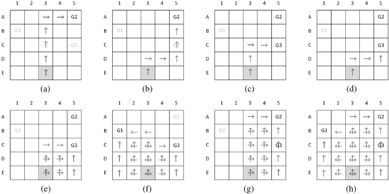
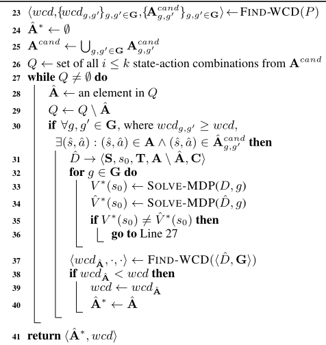
- ÷ Step 3: We first describe an unoptimized version of this step, which skips line 30, and describe the optimized version later. The algorithm evaluates each set of (up to) k state-action pairs ˆA in the candidate set Q and ensures that the removal of these state-action pairs will not
change the expected cost to reach any of the goals g 2 G (lines 27-29, 31-36). If it changes the expected cost for any goal, these state-action pairs are not considered and the algorithm iterates to the next set of state-action pairs. If it does not change the expected cost for any goal, then the algorithm computes the wcd if these state-action pairs are removed (line 37). Note that the FIND-WCD function call here should not include lines 10-13.
- ÷ Step 4: Finally, it stores the best wcd reduction and the corresponding set of state-action pairs (lines 38-40) and returns it (line 41).
We now describe the optimization on line 30 for Step 3. For each pair of distinct goals g↪ g0 2 G, the algorithm computes the wcd of a subproblem that considers only these goals and ignores all other goals (lines 18-19). This wcd value is stored in variable wcdg↪g0 . Additionally, observe that in order to reduce the wcd of the original problem, then at least one stateaction pair in candidate set Acand g↪g0 must be removed for all pairs of distinct goals g↪ g0 2 G, where wcdg↪g0 is the wcd of the original problem. Otherwise, all the original actions that can lead an agent to either goals are not removed, and the wcd will remain the same. For example, if k = 3, then removing the actions ¶(E2↪ up)↪ (D2↪ up)↪ (C2↪ up)♦ will not reduce the wcd since none of those actions are in Acand G2↪G3 and wcdG2↪G3 equals the wcd of the problem.
Theorem 2 formalizes the optimization on line 30, where the algorithm ignores candidate k state-action pairs that do not include at least one state-action pair in Acand g↪g0 for all goals g↪ g0 2 Gwhose wcdg↪g0 is greater than the current best wcd. We believe this optimization will also apply to other searchbased algorithms that searches the space of actions to reduce the wcd, such as those proposed by [Keren et al., 2014].
Theorem 2 The wcd of the problem wcd⇤ will not be reduced by removing up to k state-action pairs ˆA, where @(s↪ a) 2 ˆA : (s↪ a) 2 Acand g↪g0 ^wcdg↪g0 ≥ wcd⇤ ^ g 6= g0 .
(a) k = 1
| Domain | wcd | Runtime (s) | ||
|---|---|---|---|---|
| Instances | Reduction | R-W(≻o) | R-W(o) | |
| GRID-NA- VIGATION | 4-12-48 | 10.0!10.0 | 223 | 217 |
| IPC- GRID+ | 8-18-39 | 18.9!18.9 | 1 | 1 |
| 19-7-55 | 43.3!43.3 | 2 | 2 | |
| 9-15-44 | 4.4 ! 4.4 | 1 | 1 | |
| 5-5-4 | 4.44 ! 2.22 | 179 | 179 | |
| 10-5-4 | 13.33!11.11 | 2,097 | 2,078 | |
| 5-10-4 | 12.22!8.89 | 3,864 | 3,842 | |
| 10-10-4 | 20.00!18.89 | 112,205 | 111,842 | |
| 5-3 | 3.33 ! 3.33 | 4 | 4 | |
| BLOCK- WORDS | 6-5 | 4.44 ! 2.22 | 376 | 321 |
| 7-8 | 11.11!11.11 | 13,649 | 13,619 | |
| 7-11 | 7.78 ! 7.78 | 21,268 | 5,781 | |
| 2-2-2-2 | 6.67!6.67 | 4 | 4 | |
| LOGIS- TICS | 2-2-3-3 | 6.67!6.67 | 112 | 111 |
| 3-3-2-2 | 6.67!6.67 | 1,638 | 1,629 | |
| 3-3-3-3 | - | timeout | timeout | |
wcd Runtime (s)
(c) k = 3
wcd Runtime (s)
Reduction R-W(≻o) R-W(o)
18.9 ! 18.9
10.0 ! 8.9
43.3 ! 43.3
4.44 ! 2.22
4.4 ! 3.3
2,097 2,078 13.33!11.11
3,933 3,909
1
1
2
2
2
2
294
226
10.0 ! 8.9
43.3 ! 43.3
Reduction R-W(≻o) R-W(o)
18.9 ! 18.9
4.4 ! 3.3
46,286 46,718
1
1
3
3
5
4
1,497 1,034
3,327 3,328 13.33!11.11 30,561 31,507
4,984 4,241
10-10-4 20.00!18.89 112,205 111,842 20.00!15.56 117,207 114,449
12.22 ! 8.89
3.33 ! 3.33
-
4.44 ! 2.22
7.78 ! 7.78
6.67 ! 6.67
6.67 ! 6.67
6.67 ! 3.33
-
18
4,082
19
718
timeout timeout
timeout 159,924
4.44 ! 2.22
12.22 ! 8.89
-
35,010 20,745
timeout timeout
3.33 ! 3.33
-
4.44 ! 2.22
-
61
60
25,302 6,996
timeout timeout
timeout timeout
29
31
1,131
971
4,110 4,040
timeout timeout
6.67 ! 6.67
6.67 ! 3.33
6.67 ! 6.67
-
131
129
26,657 24,261
41,891 42,254
timeout timeout
Table 1: Experimental Results for Stochastic GRD Problems
Finally, solving S-GRDs is at least NP-hard as one of the subroutines, solving the Stochastic Longest Path (SLP) problem to compute the wcd, is NP-hard [Kolobov, 2013].
4 Experimental Results
We evaluated our REDUCE-WCD algorithm with and without the optimization on Line 30 (labeled R-W(o) and RW(≻o), respectively) on the same four deterministic benchmarks domains [Keren et al., 2014], except that we modified them to allow for stochastic actions, where each action can transition to its deterministic successor with probability 0.9 and stay in the same state with probability 0.1. The four domains are: (1) GRID-NAVIGATION, where each instance is defined by the x- and y-dimensions and the number of cells; (2) IPC-GRID+, where each instance is defined by the xand y-dimensions and the number of locks/keys; (3) BLOCKWORDS, where each instance is defined by the number of blocks and words/goals; and (4) LOGISTICS, where each instance is defined by the number of packets, places, trucks, and airplanes. Table 1 tabulates the results. The experiments were conducted on a 3.1GHz quad-core machine with 6GB of RAM and a timeout of 2 days was set.
- ÷ As expected, when k increases, the runtimes increased but the wcd was reduced in more cases. For the instances where the wcd remained unchanged, we suspect that it is because of one of the following reasons: (1) the wcd cannot be reduced further even if k = 1, or (2) the wcd can only be reduced with a significantly larger k. For the second and third GRID-NAVIGATION instances, we have empirically verified that it is the former case as there is only one optimal policy to reach each of the goal and blocking any action will result in a suboptimal policy. This is also the reason why the runtimes for these instances are very small. For the other instances, especially those with significantly larger runtimes, it may be the latter case. However, since S-GRDs are offline
problems, if a larger k is necessary, one could run the algorithm for a longer amount of time.
- ÷ GRID-NAVIGATION and IPC-GRID+ are the two domains with a larger number of instances with wcd reductions. In the BLOCK-WORDS domain, words (goals) can differ in only one letter. As a result, the goals are very similar to one another and it is difficult to reduce the wcd with small values of k. In the LOGISTICS domain, the optimal policies for the different goals are already rather distinct. As a result, it is also difficult to reduce the wcd.
- ÷ In general, the runtimes of R-W(o) are smaller than the runtimes of R-W(≻o) due to the optimization savings. These savings are up to 82%. However, the runtimes of the R-W(o) can be larger than the runtimes of R-W(≻o), indicating that in those instances, little pruning is done and time is wasted on overhead. The additional overhead results in at most 8%more runtime.
- ÷ While the runtime of R-W can be large, this is not a major concern since S-GRD problems are offline problems.
5 Conclusions and FutureWork
A new and novel approach to goal recognition is Goal Recognition Design (GRD), where the problem is to modify the underlying environment such that agents are forced to reveal their goals as early as possible. However, the GRD model and existing GRD algorithms assume that the outcomes of agent actions are deterministic. In this paper, we propose the Stochastic GRD (S-GRD) model, which subsumes GRD and allows outcomes of agent actions to be stochastic, as well as introduce an MDP-based approach to solve this problem.
For future work, we will consider other metrics aside from wcd such as those that measure the mean and variance of the distribution of the expected cost over all possible nondistinctive policy prefixes. We will also consider other possible definitions for non-distinctive policy prefixes such as those that are defined over all goals instead of pairs of goals.
Acknowledgments
We thank Sarah Keren for sharing with us her implementation of her GRD solvers. We would also like to thank all the reviewers for their constructive comments and suggestions. Finally, this research is partially supported by NSF grants 1345232 and 1550662. The views and conclusions contained in this document are those of the authors and should not be interpreted as representing the official policies, either expressed or implied, of the sponsoring organizations, agencies, or the U.S. government.
@inproceedings{ijcai2016p464,
  title     = {Goal Recognition Design with Stochastic Agent Action Outcomes},
  author    = {Wayllace, Christabel and Hou, Ping and Yeoh, William and Son, Tran Cao},
  booktitle = {Proceedings of the Twenty-Fifth International Joint Conference on
               Artificial Intelligence, {IJCAI-16}},
  publisher = {AAAI Press / International Joint Conferences on Artificial Intelligence},
  editor    = {Subbarao Kambhampati},
  pages     = {3279--3284},
  year      = {2016},
  month     = {7},
  url       = {https://ijcai.org/proceedings/2016/464},
}
TY - CPAPER TI - Goal Recognition Design with Stochastic Agent Action Outcomes AU - Wayllace, Christabel AU - Hou, Ping AU - Yeoh, William AU - Son, Tran Cao T2 - Proceedings of the Twenty-Fifth International Joint Conference on Artificial Intelligence, IJCAI-16 PB - AAAI Press / International Joint Conferences on Artificial Intelligence PY - 2016 SP - 3279 EP - 3284 UR - https://ijcai.org/proceedings/2016/464 ER -Copied
Machine-readable versions of this paper, for tools and AI agents:





