
Graph-Based Factorization of Classical Planning Problems
Proceedings of the Twenty-Fifth International Joint Conference on Artificial Intelligence. Pages 3286-3291.
Abstract
In domain-independent planning, dependencies of operators and variables often prevent the effective application of planning techniques that rely on loosely coupled problems (like factored planning or partial order reduction). In this paper, we propose a generic approach for factorizing a classical planning problem into an equivalent problem with fewer operator and variable dependencies. Our approach is based on variable factorization, which can be reduced to the well-studied problem of graph factorization. While the state spaces of the original and the factorized problems are isomorphic, the factorization offers the potential to exponentially reduce the complexity of planning techniques like factored planning and partial order reduction.
- [Alkhazraji et al., 2012] Yusra Alkhazraji, Martin Wehrle, Robert Mattmüller, and Malte Helmert. A stubborn set al- gorithm for optimal planning. In Proc. ECAI 2012, pages 891-892, 2012.
- [Amir and Engelhardt, 2003] Eyal Amir and Barbara Engel- hardt. Factored planning. In Proc. IJCAI 2003, pages 929- 935, 2003.
- [Aurenhammer et al., 1992] Franz Aurenhammer, Johann Hagauer, and Wilfried Imrich. Cartesian graph factoriza- tion at logarithmic cost per edge. Computational Complex- ity, 2:331-349, 1992.
- [Brafman and Domshlak, 2006] Ronen I. Brafman and Carmel Domshlak. Factored planning: How, when and when not. In Proc. AAAI 2006, pages 809-814, 2006.
- [Brafman and Domshlak, 2008] Ronen I. Brafman and Carmel Domshlak. From one to many: Planning for loosely coupled multi-agent systems. In Proc. ICAPS 2008, pages 28-35, 2008.
- [Bylander, 1994] Tom Bylander. The computational com- plexity of propositional STRIPS planning. Artificial In- telligence, 69(1-2):165-204, 1994.
- [Crespelle and Thierry, 2015] Christophe Crespelle and Eric Thierry. Computing the directed cartesian-product decom- position of a directed graph from its undirected decompo- sition in linear time. Discrete Mathematics, 338(12):2393- 2407, 2015.
- [Fabre et al., 2010] Eric Fabre, Loïg Jezequel, Patrik Haslum, and Sylvie Thiébaux. Cost-optimal factored planning: Promises and pitfalls. In Proc. ICAPS 2010, pages 65-72, 2010.
- [Godefroid, 1996] Patrice Godefroid. Partial-Order Meth- ods for the Verification of Concurrent Systems -An Ap- proach to the State-Explosion Problem, volume 1032 of Lecture Notes in Computer Science. Springer-Verlag, 1996.
- [Haslum et al., 2007] Patrik Haslum, Adi Botea, Malte Helmert, Blai Bonet, and Sven Koenig. Domain- independent construction of pattern database heuristics for cost-optimal planning. In Proc. AAAI 2007, pages 1007- 1012, 2007.
- [Haslum, 2007] Patrik Haslum. Reducing accidental com- plexity in planning problems. In Proc. IJCAI 2007, pages 1898-1903, 2007. IJCAI
- [Helmert, 2006] Malte Helmert. The Fast Downward plan- ning system. Journal of Artificial Intelligence Research, 26:191-246, 2006.
- [Holte et al., 2015] Robert C. Holte, Yusra Alkhazraji, and Martin Wehrle. A generalization of sleep sets based on operator sequence redundancy. In Proc. AAAI 2015, pages 3291-3297, 2015.
- [Imrich and Peterin, 2007] Wilfried Imrich and Iztok Pe- terin. Recognizing cartesian products in linear time. Dis- crete Mathematics, 307(3-5):472-483, 2007.
- [Kelareva et al., 2007] Elena Kelareva, Olivier Buffet, Jinbo Huang, and Sylvie Thiébaux. Factored planning using de- composition trees. In Proc. IJCAI 2007, pages 1942-1947, 2007. IJCAI
- [Knoblock, 1994] Craig A. Knoblock. Automatically gen- erating abstractions for planning. Artificial Intelligence, 68(2):243-302, 1994.
- [Nissim et al., 2012] Raz Nissim, Udi Apsel, and Ronen I. Brafman. Tunneling and decomposition-based state re- duction for optimal planning. In Proc. ECAI 2012, pages 624-629, 2012.
- [Sabidussi, 1960] Gert Sabidussi. Graph multiplication. Mathematische Zeitschrift, 72:446-457, 1960.
- [Seipp and Helmert, 2011] Jendrik Seipp and Malte Helmert. Fluent merging for classical planning problems. In ICAPS 2011 Workshop on Knowledge Engineering for Planning and Scheduling, pages 47-53, 2011.
- [Sievers et al., 2012] Silvan Sievers, Manuela Ortlieb, and Malte Helmert. Efficient implementation of pattern database heuristics for classical planning. In Proc. SoCS 2012, pages 105-111, 2012.
- [Valmari, 1989] Antti Valmari. Stubborn sets for reduced state space generation. In Proc. APN 1989, pages 491- 515, 1989.
- [van den Briel et al., 2007] Menkes van den Briel, Subbarao Kambhampati, and Thomas Vossen. Fluent merging: A general technique to improve reachability heuristics and factored planning. In ICAPS 2007 Workshop on Heuristics for Domain-Independent Planning, 2007.
- [Wehrle and Helmert, 2012] Martin Wehrle and Malte Helmert. About partial order reduction in planning and computer aided verification. In Proc. ICAPS 2012, 2012.
- [Wehrle and Helmert, 2014] Martin Wehrle and Malte Helmert. Efficient stubborn sets: Generalized algorithms and selection strategies. In Proc. ICAPS 2014, pages 323-331, 2014.
- [Winkler, 1987] Peter Winkler. Factoring a graph in poly- nomial time. European Journal of Combinatorics, 8:209- 212, 1987.
References were extracted automatically from the PDF and may contain errors.
Full text extracted automatically from the PDF; figures, tables and equations may differ. The PDF is the version of record.
1 Introduction
Automated planning is a computationally hard task [Bylander, 1994], and various directions to tackle this task have been proposed in the last decade. A popular direction is based on exploiting the independence of variables or operators in the formulation of the given planning problem. This direction has been (and still is) investigated for planning in many different variants and contexts, e.g., representing the core idea of factored planning [Amir and Engelhardt, 2003; Brafman and Domshlak, 2006; Kelareva et al., 2007; Brafman and Domshlak, 2008; Fabre et al., 2010] and approaches based on partial order reduction applied to planning [Alkhazraji et al., 2012; Wehrle and Helmert, 2012; Nissim et al., 2012; Wehrle and Helmert, 2014; Holte et al., 2015]. Factored planning solves subproblems individually and finally combines the resulting local solutions to a global plan. Partial order reduction explores only representatives of "permutation equivalent" sequences of independent operators. Both directions are most beneficial in "loosely coupled" problems with a high degree of variable and operator independence.
Although much research has been devoted to develop approaches that exploit independence in planning problems in a given formulation, surprisingly little research has been done on the investigation of (automated) techniques to equivalently reformulate a planning problem such that the reformulation offers fewer variable and operator dependencies. Such reformulation techniques appear to be attractive as they could render a given planning problem potentially more amenable to all approaches that benefit from "loosely coupled" problems, including the ones mentioned above. The most related paper that has addressed the task of equivalently reformulating a given planning problem in a more "factored" way is the paper by Haslum [2007]. Haslum states that "a problem formulation with less 'coupling' (fewer mutual dependencies) between variables is generally better". However, he concludes (and leaves as open questions) that how to instantiate his technique "to arrive at a better problem formulation is not [...] easy, and automating [...] even more difficult". Apparently, finding automatic techniques appears to be challenging.
In this paper, we propose a novel direction for reformulating planning problems based on variable factorization. Planning problems are usually formalized with the help of variables to describe the states of the world. We provide the theoretical basis for a generic approach to algorithmically decide how a given variable can be factorized into several independent variables and corresponding operators. We show that factorizing variables can be reduced to graph factorization, which is a well-studied problem in discrete mathematics. The resulting factorized formulation of the planning problem is equivalent to the original problem in the sense that their state spaces are isomorphic. However, due to fewer operator and variable dependencies, the factorization offers the potential to exponentially reduce the complexity of planning techniques that rely on "loosely coupled" problems.
2 Preliminaries
For a finite set of finite-domain state variables V with finite domain dom(v) for all v 2 V, we define a partial state s as a mapping from a subset vars(s) ✓ V to values in dom(v) for all v 2 vars(s). In other words, vars(s) denotes the set of variables for which the partial state s is defined. For v 62 vars(s), we say that the value of v in s is undefined, which we denote by ?. In a given partial state s, the value of v in s is s[v]. A partial state s complies with a partial state s0 if s[v] = s0 [v] for all v 2 (vars(s) \ vars(s0 )). A partial state s is called a state if vars(s) = V. We sometimes denote (partial) states by sets of variable/value assignments.
A SAS+ planning problem ⇧ = hV↪O↪ s0↪ s?i is defined in terms of a finite set of finite-domain state variables V, a finite set of operators O, an initial state s0, and a partial goal state s?. Operators o = hpre(o)↪ e↵ (o)↪ cost(o)i 2 O consist of a precondition pre(o), an effect e↵ (o), and a function cost(o). Both pre(o) and e↵ (o) are partial states, and cost(o) assigns a non-negative cost value to o. An operator o is applicable in a state s if pre(o) complies with s. Applying an applicable operator o in s yields the successor state s0 , which is obtained from s by setting the values of all v 2 vars(e↵ (o)) to e↵ (o)[v], and retaining the values of the other variables from s. We say that an operator o 2 O reads a variable v if v 2 vars(pre(o)), and that it writes to v if v 2 vars(e↵ (o)). For technical reasons (and without loss of generality), we require variables v that occur in both the precondition and the effect of o to not read v and write to v with the same value, i.e., if v 2 vars(pre(o))\vars(e↵ (o)), then pre(o)[v] 6= e↵ (o)[v].
A plan ⇡ = o1↪ ▷ ▷ ▷ ↪ on is a sequence of operators that is sequentially applicable in the initial state, and applying this sequence yields a state s that complies with s?. A plan ⇡ is optimal if the summed cost values of the operators in ⇡ are minimal among all plans in ⇧.
For each operator o 2 O and variable v 2 V, we define the partial state pre∩v(o) as pre∩v(o)[v0 ] := pre(o)[v0 ] for all v0 2 vars(pre(o)) ∩ ¶v♦, and pre∩v(o)[v0 ] as undefined for all other variables v0 . Informally, pre∩v(o) represents the partial state obtained from pre(o) when setting the value of v to undefined. Accordingly, we define e↵ ∩v(o) for e↵ (o) as the partial state obtained from e↵ (o) when setting the value of v to undefined.
For a planning problem ⇧ = hV↪O↪ s0↪ s?i, the state space of ⇧ is defined as the transition system T ⇧ = (S↪ L↪ T↪ s0↪ S?), where S is the set of states of ⇧, L is the set ¶l(o) ♣ o 2 O♦ of operator labels induced by O, T ✓ S ⇥ L ⇥ S is the set of transitions with (s↪ l(o)↪ s0 ) 2 T if o is applicable in s and yields the successor state s0 , s0 is the initial state of ⇧, and S? is the set of goal states that comply with s?. For a variable v 2 V, we define the atomic transition system T v of v as the homomorphic projection of T ⇧ to v via the abstraction function ↵(s) := s[v], i.e., as the directed graph T v = hSv ↪ L↪ T v ↪ sv0 ↪ Sv ? i with Sv = dom(v), T v = ¶(↵(s)↪ l(o)↪ ↵(s0 )) ♣ (s↪ l(o)↪ s0 ) 2 T♦, sv0 = ↵(s0), and Sv ? = ¶↵(s) ♣ s 2 S?♦.
2.1 Graph Factorization
In discrete mathematics, the factorization of graphs has been studied intensively since the 1960s, both for undirected and directed graphs, and for different kinds of products. A factorization of a graph G is given by graphs G1↪ ▷ ▷ ▷ ↪ Gn such that the product of G1↪ ▷ ▷ ▷ ↪ Gn yields G. More specifically, it has been shown that undirected and directed graphs without selfloops have a unique factorization into prime graphs with respect to the Cartesian product, and that this factorization can be computed in polynomial time [Sabidussi, 1960; Winkler, 1987; Aurenhammer et al., 1992; Imrich and Peterin, 2007]. Recently, a linear factorization algorithm for directed graphs without self-loops has been proposed [Crespelle and Thierry, 2015]. For directed graphs G1 = hV1↪E1i↪ ▷ ▷ ▷ ↪Gm = hVm↪Emi, the Cartesian product of G1↪ ▷ ▷ ▷ ↪Gm is defined as G⇥ := hV ⇥↪ E⇥i, with V ⇥ := V1 ⇥ · · · ⇥ Vm. There is an edge hhv1↪ ▷ ▷ ▷ ↪ vmi↪ hw1↪ ▷ ▷ ▷ ↪wmii 2 E⇥ if and only if there is i 2 ¶1↪ ▷ ▷ ▷ ↪m♦ with hvi↪wii 2 Ei and vj = wj for all j 6= i. We remark that, in contrast to synchronized products, edges in Cartesian products are not synchronized across different graphs, in the sense that every edge in the product G⇥ corresponds to exactly one vertex change in one graph Gi. In the following, we propose a factorization approach for planning problems based on a reduction to Cartesian graph factorization.
3 AMotivating Example
Assume that a truck is supposed to drive from its initial location 1 to its goal location 4, where the goal location can be reached via the intermediate locations 2 or 3. A straightforward formulation in STRIPS will include four variables at-i with i 2 ¶1↪ 2↪ 3↪ 4♦ to represent the location of the truck. In SAS+, one variable pos with domain dom(pos) = ¶1↪ 2↪ 3↪ 4♦ will typically be used. Figure 1 shows the atomic transition system of the SAS+ version (left).
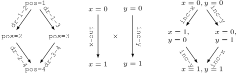
Both the STRIPS and the SAS+ formulation are "tightly coupled" in the sense that, e.g., partial order reduction will not provide any reduction: Partial order reduction is a pruning method that eliminates permutations of sequences of independent operators that lead to goal states, such that at least one permutation thereof is preserved. In the example, partial order reduction does not prune anything because the two alternative paths from locations 1 to 4 over 2 or 3 are not spanned by the same set of operators, i.e., there is no equivalent permutation of operator sequences.
However, there exists a factorization of the SAS+ variable pos into SAS+ variables x and y with dom(x) = dom(y) = ¶0↪ 1♦, with operators inc-x and inc-y that set x and y from 0 to 1, respectively. Figure 1 shows the corresponding factorized graphs representing x and y in the middle. Extending Cartesian products to labeled graphs in the straight forward way (we will formalize this below), we observe that the Cartesian product of the two factorized graphs (shown on the right in Figure 1) is structurally isomorphic to the atomic transition system in the original formulation, leaving operator names aside for the moment. This means that we can capture the semantics of the original formulation with the factorized one. At the same time, the factorized formulation yields independent operators than can be permuted arbitrarily. Hence, one of the two permutations of the plans (inc-x,inc-y and inc-y,inc-x) can be eliminated by the use of partial order reduction. To summarize, we observe that the factorization can yield a decoupled, but equivalent semantics of the original planning problem, and there is a 1:1 correspondence of the plans in the two formulations.
4 Factorization of Planning Problems
In the following, we will generalize the concept of Cartesian graph factorization of unlabeled graphs to transition systems. The following definitions consider transition systems without self-loops - we will discuss how to handle self-loops (as they occur in atomic transition systems of planning problems) below. We start by defining Cartesian products. To keep things simple, we restrict the definitions to two graphs (the generalization to an arbitrary number is straight forward).
Definition 1 (Cartesian Product). Let G1 = (S1 ↪ L↪ T 1 ↪ s10 ↪ S1 ? ) and G2 = (S2 ↪ L↪ T 2 ↪ s20 ↪ S2 ? ) be transition systems with common label set L and without self-loops (i.e., without transitions of the form (s↪ l↪ s) for any state s and any label l). The Cartesian product G1 ⇥G2 of G1 and G2 is the transition system G⇥ := (S⇥↪ L↪ T ⇥↪ s⇥0 ↪ S⇥ ? ), where S⇥ = ¶(s1 ↪ s2 ) ♣ s1 2 S1 ↪ s2 2 S2 ♦ is the Cartesian product of S1 and S2 , and there is an edge ((s1 ↪ s2 )↪ l↪ (t1 ↪ t2 )) in T ⇥ iff (s1 ↪ l↪ t1 ) 2 T 1 and s2 = t2 , or s1 = t1 and (s2 ↪ l↪ t2 ) 2 T 2 . Analogously to S⇥, s⇥0 is defined as (s10 ↪ s20 ), and S⇥ ? as the Cartesian product of S1 ? and S2 ? .
Definition 2 (Cartesian Factor). Let G = (S↪ L↪ T↪ s0↪ S?) be a transition system without self-loops. The transition systems G1 = (S1 ↪ L↪ T 1 ↪ s10 ↪ S1 ? ) and G2 = (S2 ↪ L↪ T 2 ↪ s20 ↪ S2 ? ) are Cartesian factors of G iff G is isomorphic to the Cartesian product G⇥ = (S⇥↪ L↪ T ⇥↪ s⇥0 ↪ S⇥ ? ) of G1 and G2, i.e., iff there is a bijective function ' : S ! S⇥ such that hs↪ l↪ ti 2 T iff h'(s)↪ l0 ↪ '(t)i 2 T ⇥ for l↪ l0 2 L.
We remark that in Def. 2, two transition systems are called "isomorphic" if their graph structures are isomorphic in the usual sense, whereas labels (that correspond to operator names when used for planning problems) are allowed to be different.
We now apply the concept of graph factorization to planning. As atomic transition systems characterize the behavior of variables, values, and value changes, a factorization of such an atomic transition system T v of variable v corresponds to a factorization of v itself. Furthermore, the factorized variables of v also yield a factorization of the operators that read or write to v. To formally define these factorized operators, let us come back to the question how to handle selfloops in atomic transition systems. We observe that, apart from the trivial case where an operator does not mention variable v at all, self-loops in an atomic transition system T v can either be induced by an operator that reads v, but does not write to v, or vice versa does not read v, but writes to v. In the following definition of factorized operators, these cases are handled separately from the case where an operator both reads and writes to v. For a given atomic transition system T v = hSv ↪ L↪ T v ↪ sv0 ↪ Sv ? i, we define the atomic transition system without self-loops T v = hSv ↪ L↪ T v ↪ sv0 ↪ Sv ? i, which is obtained from T v by removing all self-loops from T v , i.e., T v := ¶(s↪ l↪ t) 2 T v ♣ s 6= t♦.
Let Ov := ¶o 2 O♣v 2 (vars(pre(o)) [ vars(e↵ (o)))♦ be the operators that "work on v". In the following, we again restrict our definitions to two graphs to keep things simple.
Definition 3 (Factorized Operators). Let ⇧ = hV↪O↪ s0↪ s?i be a planning problem, let v 2 V be a variable with atomic transition system T v = hSv ↪ L↪ T v ↪ sv0 ↪ Sv ? i, and let T v = hSv ↪ L↪ T v ↪ sv0 ↪ Sv ? i be the corresponding atomic transition system without self-loops. Let T v1 = hSv1 ↪ L↪ T v1 ↪ sv1 0 ↪ Sv1 ? i and T v2 = hSv2 ↪ L↪ T v2 ↪ sv2 0 ↪ Sv2 ? i be Cartesian factors of T v and let ' be the bijection between T v and T v1 ⇥ T v2 = (S⇥↪ L↪ T ⇥↪ s⇥0 ↪ S⇥ ? ).
Let o = hpre(o)↪ e↵ (o)↪ cost(o)i be an operator with o 2 Ov . The factorized operator of of o is defined as follows. We distinguish three cases.
- v 2 vars(pre(o)) \ vars(e↵ (o)), i.e., o both reads and writes to v. Then o induces a transition (pre(o)[v]↪ l↪ e↵ (o)[v]) 2 T v , which, via ', corresponds to a transition t⇥ = ((s1↪ s2)↪ l0 ↪ (t1↪ t2)) 2 T ⇥ for some l0 2 L, where (s1↪ s2) = '(pre(o)[v]) and (t1↪ t2) = '(e↵ (o)[v]). By the definition of Cartesian products, the transition t⇥ is induced by exactly one transition (si↪ l0 ↪ ti) 2 T vi for some i 2 ¶1↪ 2♦. The factorized operator of o is defined as
with co := cost(o).
- v 2 vars(pre(o)) ∩ vars(e↵ (o)), i.e., o only reads v, but does not write to v. Let '(pre(o)[v]) = (s1↪ s2). The factorized operator of o is defined as
i.e., the condition ¶v 7! pre(o)[v]♦ is replaced by the corresponding conditions on the factorized variables and values obtained from '.
- v 2 vars(e↵ (o)) ∩ vars(pre(o)), i.e., o only writes to v, but does not read v. Let '(e↵ (o)[v]) = (t1↪ t2). The factorized operator of o is defined as
i.e., the effect ¶v 7! e↵ (o)[v]♦ is replaced by the corresponding effects on the factorized variables and values obtained from '.
Bullet point 1 in Def. 3 refers to operators that both read and write to v and hence induce a non-self-loop transition in the atomic transition system T v (recall that we assume pre(o)[v] 6= e↵ (o)[v] for o). Such operators are mapped to factorized operators that only read and write to only one factorized variable, and retain the precondition and effects on the remaining variables. Bullet points 2 and 3 in Def. 3 cover the remaining cases where o only reads v or writes to v, respectively. Such operators can only induce self-loops, hence they are not captured by the factorization (which ignores self-loops). The corresponding factorized operator is defined based on the variable/value combination of the factorized variables and the bijective mapping provided by '.
We note that, due to the definition of Cartesian products, there are generally several operators that are mapped to the same factorized operator. For example, in the planning problem in Fig. 1, the two operators that drive from position 1 to 2 and drive from position 3 to 4, are mapped to the single operator that sets x from 0 to 1.
We are now ready to define factorized planning problems (for simplicity, again restricted to the case of two factors).
Definition 4 (Factorized Planning Problem). Let ⇧ = hV↪O↪ s0↪ s?i be a planning problem, let v 2 V be a variable with atomic transition system T v , and let v1↪ v2 be factorized variables of v, i.e., let T vi = hSvi ↪ L↪ T vi ↪ svi 0 ↪ Svi ? i for i 2 ¶1↪ 2♦ be Cartesian factors of T v and let ' be the bijection between T v and T v1 ⇥ T v2 . The factorized planning problem ⇧f = hV f ↪ Of ↪ sf0 ↪ sf? i with respect to v1↪ v2 is defined as follows:
- V f := V ∩ ¶v♦ [ ¶v1↪ v2♦ with ¶v1↪ v2♦ \V = ;, where dom(vi) := Svi for i 2 ¶1↪ 2♦.
- Let s0[v] = x and '(x) = (x1↪ x2). Then sf0 [vi] := xi for i 2 ¶1↪ 2♦, and sf0 [w] := s0[w] for all w 2 V ∩ ¶v♦.
- Of := ¶of factorized operator of o ♣ o 2 Ov ♦[O∩Ov
- If v ◁2 vars(s?), then sf?[vi] := ? for i 2 ¶1↪ 2♦. Otherwise, let s?[v] = x and '(x) = (x1↪ x2). Then sf? [vi] := xi for i 2 ¶1↪ 2♦. In both cases, sf?[w] := s?[w] for all w 2 V ∩ ¶v♦.
We remark that the definition of factorized planning problems is solely based on the bijective mapping from variable assignments ¶v 7! x♦ to factorized assignments ¶v1 7! x1↪ v2 7! x2♦ provided by ' (i.e. '(x) = (x1↪ x2)). As a consequence, the state space graphs of original and factorized problems are isomorphic (modulo operator renaming), which we show formally in the following theorem. We again only consider the case of two factors for simplicity.
Theorem 1. Let ⇧ = hV↪O↪ s0↪ s?i be a planning problem, v 2 V, and v1↪ v2 be factorized variables of v induced by an isomorphism ' in the sense of Def. 2. Let ⇧f = hV f ↪Of ↪ sf0 ↪ sf?i be the factorized planning problem with respect to v1↪ v2. Then the state space graphs of ⇧ and ⇧f are isomorphic (where operators can have different names).
Proof. Let T v , T v1 and T v2 be the atomic transition systems (without self-loops) of v↪ v1↪ v2. Let S and S f be the set of states of ⇧ and ⇧f . In the following, for a tuple '(x) = (x1↪ x2), we denote the ith component xi of '(x) by '(x)[i], i 2 ¶1↪ 2♦. We will show that the state spaces of ⇧ and ⇧f are isomorphic via the function : S[O!S f [Of , which is defined by
for states, by (o) := of for o 2 Ov and (o) := o for o 2 O ∩ Ov . For brevity, we only consider the non-trivial case for operators o 2 Ov . Assume there is a state transition from state s to t by applying such o in the state space of ⇧. We will show that there is a corresponding state transition from (s) to (t) by applying (o) = of in the state space of ⇧f .
- v 2 vars(pre(o)) \ vars(e↵ (o)). To simplify notation, let x := s[v] and y := t[v], with x 6= y. As o sets v from x to y, there is a transition hx↪ l↪ yi in T v . As ' is an isomorphism between T v and the Cartesian product T ⇥ of T v1 and T v2 , there is a transition t⇥ := h'(x)↪ l0 ↪ '(y)i in T ⇥ for some l0 2 L. By the definition of Cartesian products, the transition t⇥ is induced by a transition in exactly one Cartesian factor i 2 ¶1↪ 2♦, say factor i. Hence there is a transition h'(x)[i]↪ l0 ↪ '(y)[i]i in T vi . This is the defining transition of operator of according to Def. 3: of = hpre∩v(o) [ ¶vi 7! '(x)[i]♦; e↵ ∩v(o) [ ¶vi 7! '(y)[i]♦; cost(o)i. It follows that of is applicable in (s) and leads to (t): of sets vi from '(x)[i] to '(y)[i], and o and of have the same preconditions and effects on other variables than v (hence pre(of ) and e↵ (of ) comply with (s) and (t), respectively).
- v 2 vars(pre(o)) ∩ vars(e↵ (o)). As o is applicable in s, pre(o)[v] = s[v]. By the definitions of of and , pre(of )[vi] = '(s[v])[i] = (s)[vi] for i 2 ¶1↪ 2♦, and the preconditions of of on other variables than v1↪ v2 are the same as those of o. Hence, of is applicable in (s). As o does not modify v, of does not modify v1↪ v2 either, and the effects of of on other variables than v1↪ v2 are the same as those of o. Hence, because o leads from s to t, the application of of in (s) leads to (t).
- v 2 vars(e↵ (o)) ∩ vars(pre(o)). As v does not occur in the precondition of o, of does not mention v1↪ v2 in its precondition either, and its preconditions on other variables than v1↪ v2 are the same as those of o. Hence, because o is applicable in s, of is applicable in (s). Because the application of o in s yields t, it follows that t[v] = e↵ (o)[v]. By the definitions of of and , e↵ (of )[vi] = '(t[v])[i] = (t)[vi] for i 2 ¶1↪ 2♦, and the effects of of on other variables than v1↪ v2 are the same as those of o. Hence the application of of in (s) leads to (t).
Showing that for all state transitions in ⇧f there is a corresponding transition in ⇧ is done analogously.
Corollary 1. Factorizing planning problems via isomorphism ' preserves plan existence and optimal plan cost.
Proof. Plan existence is preserved because the state spaces of the planning problems are isomorphic according to Theorem 1, and because ' preserves the initial state and goal states: goal states are preserved because v is a goal variable in the original planning problem with goal value s?[v] = x iff the factorized variables v1↪ v2 of v are goal variables in the factorized planning problem with goal values s?[vi] = '(x)[i] for i 2 ¶1↪ 2♦. Analogously, ' preserves the initial state. Optimal plan cost are preserved because factorized operators have the same cost as the corresponding operators in the original problem.
The mapping from operators O to factorized operators Of (Def. 3) allows us to transform plans ⇡f in the factorized planning problem ⇧f to plans ⇡ in the original problem ⇧ by scanning ⇡f , and "mapping back" all factorized operators in Of to operators in O. As mentioned above, assuming v to be a variable factorized into v1↪ ▷ ▷ ▷ ↪ vn, and assuming of to be a factorized operator, there are several operators in the original problem that correspond to of , hence the inverse function is not uniquely defined. However, as the state spaces of the original and the factorized problem are isomorphic, there is exactly one original operator that corresponds to of .
5 Properties of Factorized Planning Problems
We now study some properties of factorized planning problems. Brafman and Domshlak [2006] presented a factored planning algorithm whose runtime is exponential only in the treewidth of the (undirected) causal graph [Knoblock, 1994] of the planning problem and its local width, the smallest number k such that a plan that writes to each variable at most k times exists. We show that factorization can be very beneficial for factored planning.
Theorem 2. Let ⇧ be a planning problem and ⇧f be a factorized planning problem of ⇧. The runtime bound for factored planning in ⇧f can be exponentially smaller than for ⇧.
Proof. Consider a family of planning problems ⇧n (n 2 N) obtained by generalizing the example in Fig. 1. Let ⇧n consist of one variable pos with dom(pos) = ¶1↪ ▷ ▷ ▷ ↪ 2n ♦ such that the corresponding factorized planning problem ⇧fn consists of n variables v1↪ ▷ ▷ ▷ ↪ vn. For each vi, there is exactly one operator in ⇧fn that sets vi from 0 to 1 (and hence, there are n atomic transition systems with two locations, as shown in the middle in Fig. 1 for n = 2). The initial and the goal states are given by vi = 0 and vi = 1 for all i 2 ¶1↪ ▷ ▷ ▷ ↪ n♦, respectively. For all n 2 N, there is a plan in ⇧fn that affects every variable vi only once (local width 1), whereas every plan in ⇧n affects pos at least n times (local width n). The tree width of the causal graph is equal to 1 in both ⇧n and ⇧fn . Hence factored planning provides an exponential runtime bound for ⇧n but a polynomial one for ⇧fn .
In the following, we show that similar results hold for strong stubborn sets [Valmari, 1989; Alkhazraji et al., 2012] and sleep sets [Godefroid, 1996; Holte et al., 2015].
For a given state s, strong stubborn sets can prune permutations of operator sequences that consist of independent operators and lead from s to a goal state, with the guarantee that at least one of these permutations is preserved in s. Operators o and o0 are denoted as independent if o does not disable o0 (i.e., there is no variable v such that e↵ (o)[v] 6= pre(o0 )[v]), and o0 does not disable o, and o↪ o0 do not have conflicting effects (i.e., there is no variable v such that e↵ (o)[v] 6= e↵ (o0 )[v]).
Theorem 3. Let ⇧ be a planning problem and ⇧f be a factorized planning problem of ⇧. The size of the reachable state space with strong stubborn sets in ⇧f can be exponentially smaller than the corresponding size in ⇧.
Proof. Consider again the problems ⇧n and factorized problems ⇧fn from the proof of Theorem 2. In every state of ⇧fn , strong stubborn sets contain only one of the operators of ⇧fn (all factorized operator pairs are independent). This yields a reachable state space of size n + 1. In contrast, strong stubborn sets do not prune in ⇧n because all operators are not independent with each other. Hence, ⇧n has 2n reachable states.
Sleep sets are usually applied in tree search algorithms to avoid exploring equal states reached via different paths in the state space. Sleep sets can prune state transitions induced by commutative operators. Operators o and o0 are denoted as commutative if o and o0 are independent, and additionally, o and o0 do not enable each other (i.e., there is no variable v such that e↵ (o)[v] = pre(o0 )[v], and vice versa).
Theorem 4. Let ⇧ be a planning problem and ⇧f be a factorized planning problem of ⇧. The number of generated nodes with iterative deepening search and sleep sets can be exponentially smaller in ⇧f than in ⇧.
Proof. Consider the problems ⇧n and factorized problems ⇧fn from the proof of Theorem 2. Optimal plans in ⇧n and ⇧fn have length n, and therefore iterative deepening search explores all paths of length n - 1 in the second last iteration. Without pruning, ⇧n and ⇧fn have n! paths of length (n - 1) from the initial state.
Sleep set pruning in ⇧n does not prune any search node because there is no pair of operators that is commutative. Hence n! search nodes are generated at depth n - 1.
In contrast, sleep set pruning in ⇧fn prunes all but one path to every reachable state: Because operators in this problem are commutative, sleep sets assume an (arbitrary) total order < on the set of operators, and it is easy to see that under this restriction, every state can only be reached by a single path. This results in a runtime bound of O(2n ) when searching ⇧fn , an exponential reduction compared to n! for ⇧n.
6 Discussion
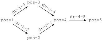
Our approach provides the basic theory of a novel direction for problem reformulation. As shown in the previous section, techniques that rely on "loosely coupled" problems can benefit from factorization. However, we also observe that the current theory for factorizing atomic transition systems such that the resulting state spaces are isomorphic is stronger than needed, as we only need the reachable part of the product to be equal to the original. Consider the example in Fig. 2, an extension of the example in Fig. 1.
The example shows an atomic transition system T , where a truck is supposed to drive from location 1 to 5 via one of the locations 2 or 3. Again, typical partial order reduction methods do not fire in this problem formulation because all pairs of operators interfere (i.e., they are not independent). However, although T cannot be factorized into non-trivial Cartesian factors, there exists a factorization into variables x, y, z and corresponding operators o1 = h¶x 7! 0♦; ¶x 7! 1♦i, o2 = h¶y 7! 0♦; ¶y 7! 1♦i and o3 = h¶x 7! 1↪ y 7! 1♦; ¶z 7! 1♦i such that the reachable state space (with the initial state ¶x 7! 0↪ y 7! 0↪ z 7! 0♦) induced by o1↪ o2↪ o3 is isomorphic to T . We observe that o1↪ o2↪ o3 are independent, which can be exploited by, e.g., partial order reduction. How to compute such "relaxed factorizations" remains an open question.
Factorizing variables into an equivalent problem formulation can be viewed as a variant of "inverse fluent merging". Fluent merging [van den Briel et al., 2007; Seipp and Helmert, 2011] merges several variables to a joint new variable with corresponding variable domain. As a result, the merged formulation can be more amenable to the computation of accurate heuristics. On the other hand, fluent merging can increase coupling in the problem formulation.
7 Towards a Planning Algorithm
Factorization algorithms for planning need to handle labeled transitions, while existing graph factorization algorithms do not handle transition labels (see Section 2.1). A straightforward, yet rather restrictive way to still make use of these algorithms is based on a try-and-check approach: Given a planning problem ⇧ and a variable v of ⇧, such an algorithm considers the atomic transition system T v , and computes a factorization of the underlying directed graph without selfloops T v where labels are ignored. To obtain a correct factorization according to our theory, the algorithm then needs to check if operators that are supposed to be mapped to the same factorized operator as defined by the Cartesian factors have the same preconditions and effects on other variables than v in ⇧. If this is the case, the factorized planning problem ⇧f can be computed. The Cartesian graph factorization can be achieved in linear time [Crespelle and Thierry, 2015]. The remaining part of checking the conditions on the factorized operators can be done in low-order polynomial time in the compact size of the planning problem, yielding an overall low-order polynomial time complexity. In addition, atomic transition systems for typical planning problems often have rather small sizes, hence the overhead of checking for Cartesian factors will mostly be negligible.
Currently, we do not have a fully automatic implementation. A preliminary analysis of planning domains from the international planning competitions up to 2014 revealed that some domains (Floortile, Grid, Sokoban, Tetris and Visitall) contain atomic transition systems whose unlabeled graph structure can be factorized. However, they do not pass the tryand-check approach, i.e., cannot be factorized into non-trivial Cartesian factors according to our theory.
As a proof of concept, we slightly modified the IPC Visitall domain such that "moving" and "marking as visited" are represented by different operators. We applied the Fast Downward planner [Helmert, 2006] to this domain and its factorization, using A⇤ with strong stubborn sets as well as IDA⇤ with sleep sets. While the factorization does not yield additional pruning with strong stubborn sets (as "moving" can still disable "mark-as-visited"), it does when applied with sleep sets. We compare IDA⇤ with and without sleep sets, using Fast Downward's blind heuristic and Fast Downward's implementation of iPDB [Haslum et al., 2007; Sievers et al., 2012]. Table 1 shows the resulting number of generated nodes (without the last f-layer to avoid tiebreaking issues) and the runtime in seconds.
| original formulation | factorized formulation | |||||||
|---|---|---|---|---|---|---|---|---|
| #nodes | runtime | #nodes | runtime | |||||
| size | nop | prune | nop | prune | nop | prune | nop | prune |
| blind | ||||||||
| 6 | 3853 | 3853 | 0.0 | 0.0 | 3853 | 987 | 0.0 | 0.0 |
| 9 | 2.5e+6 | 2.5e+6 | 12.2 | 14.4 | 2.5e+6 | 93613 | 12.2 | 0.6 |
| 12 | - | - | - | - | - | 1.1e+7 | - | 86.0 |
| iPDB | ||||||||
| 12 | 81042 | 81042 | 0.7 | 0.8 | 72721 | 19102 | 4.5 | 4.2 |
| 16 | 1.9e+7 | 1.9e+7 | 112.6 | 125.5 | 1.3e+7 | 1.5e+6 | 107.7 | 22.9 |
| 20 | - | - | - | - | - | 1.6e+8 | - | 1710.8 |
Focusing on the results with the blind heuristic (to measure the pure pruning ability on the factorization) displayed in the upper part, we observe that the factorization allows sleep sets to cut down the number of generated nodes by avoiding the generation of duplicates. The smaller search space translates into lower runtime. When using iPDB (lower part), we observe that the factorization causes iPDB to compute a more accurate heuristic (i.e., fewer nodes are generated on the factorized formulation also when no pruning is applied), which results in a slightly higher precomputation time. More importantly, we again observe that the factorization can be beneficial when applied with sleep sets, which can in turn result in fewer generated nodes and lower runtime.
8 Conclusions
We have proposed a theory for equivalently reformulating planning problems based on Cartesian graph factorization. Factorized planning problems offer the potential to yield exponentially smaller state spaces when factored planning or partial order reduction is applied. In the future, it will be important to turn the theory into practice: As we have observed, the requirement for the resulting state spaces to be isomorphic is stronger than needed, because we only need the reachable part of the product to be equal to the original. Furthermore, it will be important to investigate more sophisticated factorization algorithms for labeled graphs.
Acknowledgments
This work was supported by the Swiss National Science Foundation (SNSF) as part of the project "Automated Reformulation and Pruning in Factored State Spaces (ARAP)".
@inproceedings{ijcai2016p465,
  title     = {Graph-Based Factorization of Classical Planning Problems},
  author    = {Wehrle, Martin and Sievers, Silvan and Helmert, Malte},
  booktitle = {Proceedings of the Twenty-Fifth International Joint Conference on
               Artificial Intelligence, {IJCAI-16}},
  publisher = {AAAI Press / International Joint Conferences on Artificial Intelligence},
  editor    = {Subbarao Kambhampati},
  pages     = {3286--3291},
  year      = {2016},
  month     = {7},
  url       = {https://ijcai.org/proceedings/2016/465},
}
TY - CPAPER TI - Graph-Based Factorization of Classical Planning Problems AU - Wehrle, Martin AU - Sievers, Silvan AU - Helmert, Malte T2 - Proceedings of the Twenty-Fifth International Joint Conference on Artificial Intelligence, IJCAI-16 PB - AAAI Press / International Joint Conferences on Artificial Intelligence PY - 2016 SP - 3286 EP - 3291 UR - https://ijcai.org/proceedings/2016/465 ER -Copied
Machine-readable versions of this paper, for tools and AI agents:





